9. Supervised Learning

9.1. Classification

When response is a categorical value.

9.1.1. K Nearest Neighbours (KNN)

www.mathworks.com

Note

1. Distance Metric: Eclidean Distance (default). In sklearn it is known as (Minkowski with p = 2)
2. How many nearest neighbour: k=1 very specific, k=5 more general model. Use nearest k data points to determine classification
3. Weighting function on neighbours: (optional)
4. How to aggregate class of neighbour points: Simple majority (default)

#### IMPORT MODULES ####
import pandas as pd
import numpy as np
from sklearn.cross_validation import train_test_split
from sklearn.neighbors import KNeighborsClassifier



#### TRAIN TEST SPLIT ####
X_train, X_test, y_train, y_test = train_test_split(X, y, random_state=0)



#### CREATE MODEL ####
knn = KNeighborsClassifier(n_neighbors = 5)



#### FIT MODEL ####
knn.fit(X_train, y_train)
#KNeighborsClassifier(algorithm='auto', leaf_size=30, metric='minkowski',
#     metric_params=None, n_jobs=1, n_neighbors=5, p=2,
#     weights='uniform')



#### TEST MODEL ####
knn.score(X_test, y_test)
0.53333333333333333

9.1.2. Decision Tree

Uses gini index (default) or entropy to split the data at binary level.

Strengths: Can select a large number of features that best determine the targets.

Weakness: Tends to overfit the data as it will split till the end. Pruning can be done to remove the leaves to prevent overfitting but that is not available in sklearn. Small changes in data can lead to different splits. Not very reproducible for future data (see random forest).

More more tuning parameters https://medium.com/@mohtedibf/indepth-parameter-tuning-for-decision-tree-6753118a03c3

###### IMPORT MODULES #######
import pandas as pd
import numpy as np
from sklearn.tree import DecisionTreeClassifier



#### TRAIN TEST SPLIT ####
train_predictor, test_predictor, train_target, test_target = \
train_test_split(predictor, target, test_size=0.25)

print test_predictor.shape
print train_predictor.shape
(38, 4)
(112, 4)



#### CREATE MODEL ####
clf = DecisionTreeClassifier()



#### FIT MODEL ####
model = clf.fit(train_predictor, train_target)
print model
DecisionTreeClassifier(class_weight=None, criterion='gini', max_depth=None,
            max_features=None, max_leaf_nodes=None, min_samples_leaf=1,
            min_samples_split=2, min_weight_fraction_leaf=0.0,
            presort=False, random_state=None, splitter='best')



#### TEST MODEL ####
predictions = model.predict(test_predictor)

print sklearn.metrics.confusion_matrix(test_target,predictions)
print sklearn.metrics.accuracy_score(test_target, predictions)*100, '%'
[[14  0  0]
 [ 0 13  0]
 [ 0  1 10]]
97.3684210526 %


#### SCORE MODEL ####
# it is easier to use this package that does everything nicely for a perfect confusion matrix
from pandas_confusion import ConfusionMatrix
ConfusionMatrix(test_target, predictions)
Predicted   setosa  versicolor  virginica  __all__
Actual
setosa          14           0          0       14
versicolor       0          13          0       13
virginica        0           1         10       11
__all__         14          14         10       38



####### FEATURE IMPORTANCE #### ####
f_impt= pd.DataFrame(model.feature_importances_, index=df.columns[:-2])
f_impt = f_impt.sort_values(by=0,ascending=False)
f_impt.columns = ['feature importance']
f_impt
petal width (cm)      0.952542
petal length (cm)     0.029591
sepal length (cm)     0.017867
sepal width (cm)      0.000000

Viewing the decision tree requires installing of the two packages conda install graphviz & conda install pydotplus.

from sklearn.externals.six import StringIO
from IPython.display import Image
from sklearn.tree import export_graphviz
import pydotplus
dot_data = StringIO()
export_graphviz(dtree, out_file=dot_data,
                filled=True, rounded=True,
                special_characters=True)
graph = pydotplus.graph_from_dot_data(dot_data.getvalue())
Image(graph.create_png())

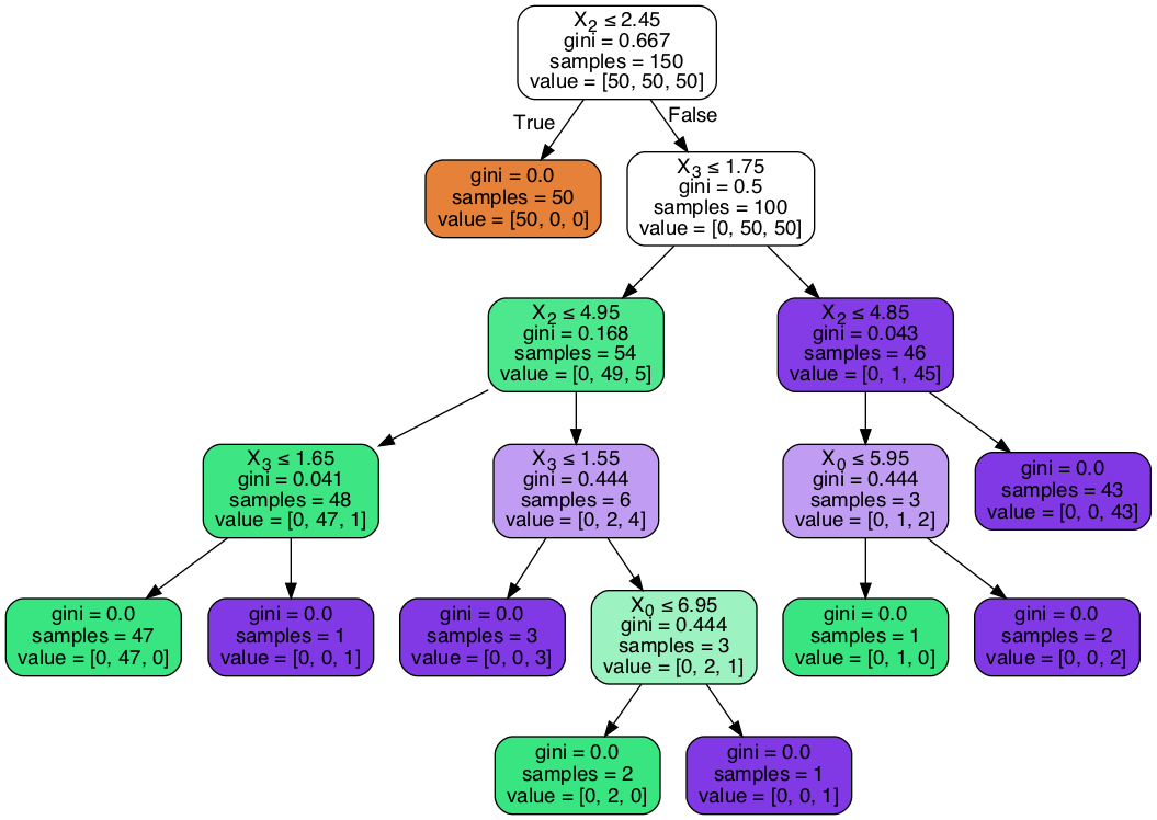
Parameters to tune decision trees include maxdepth & min sample leaf.

from sklearn.tree import DecisionTreeClassifier
from adspy_shared_utilities import plot_decision_tree
from adspy_shared_utilities import plot_feature_importances

X_train, X_test, y_train, y_test = train_test_split(X_cancer, y_cancer, random_state = 0)

clf = DecisionTreeClassifier(max_depth = 4, min_samples_leaf = 8,
                            random_state = 0).fit(X_train, y_train)

plot_decision_tree(clf, cancer.feature_names, cancer.target_names)

9.1.3. Ensemble Learning

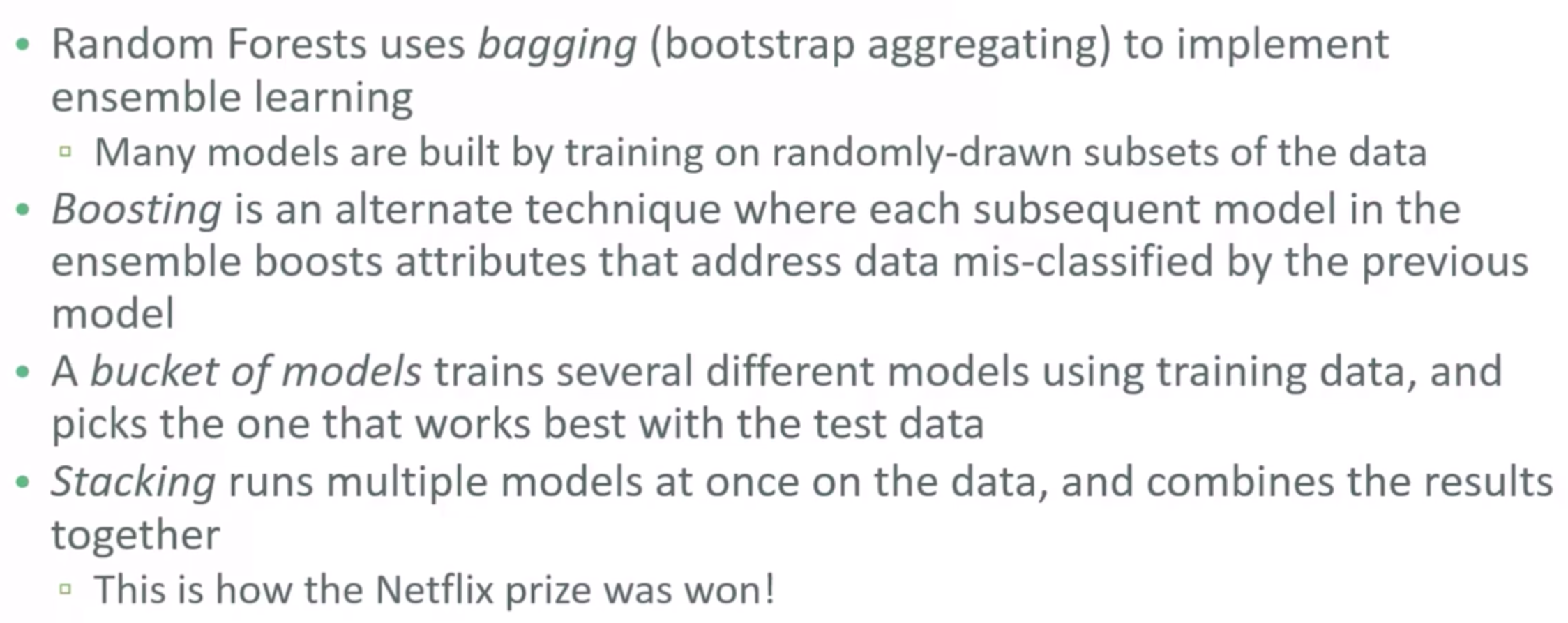
Udemy Machine Learning Course by Frank Kane

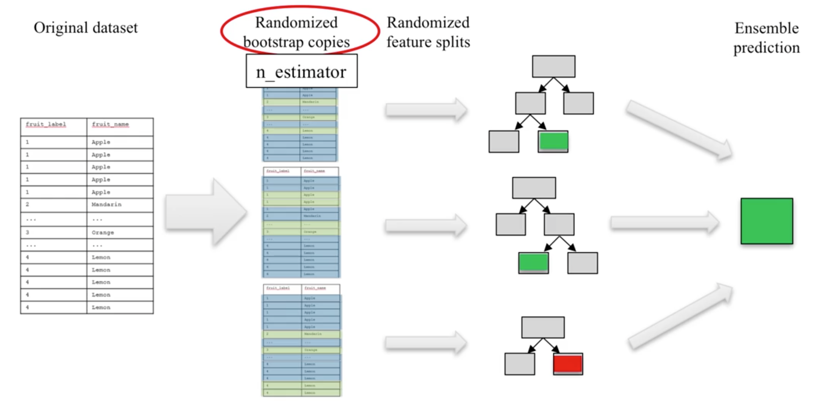
9.1.4. Random Forest

An ensemble of decision trees.

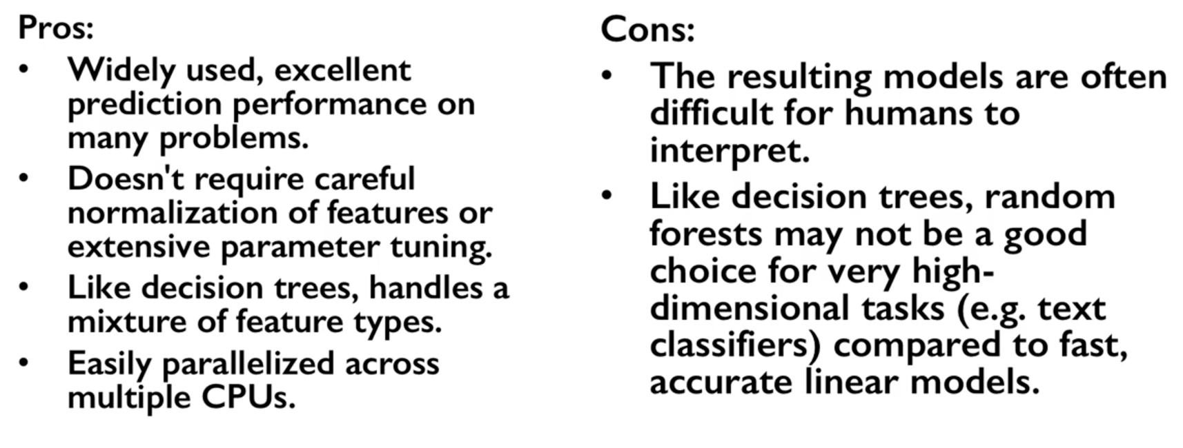
• It is widely used and has very good results on many problems

• sklearn.ensemble module

  • Classification: RandomForestClassifier
  • Regression: RandomForestRegressor

• One decision tree tends to overfit
• Many decision trees tends to be more stable and generalised
• Ensemble of trees should be diverse: introduce random variation into tree building

University of Michigan: Coursera Data Science in Python

Randomness is introduced by two ways:

• Bootstrap: AKA bagging. If your training set has N instances or samples in total, a bootstrap sample of size N is created by just repeatedly picking one of the N dataset rows at random with replacement, that is, allowing for the possibility of picking the same row again at each selection. You repeat this random selection process N times. The resulting bootstrap sample has N rows just like the original training set but with possibly some rows from the original dataset missing and others occurring multiple times just due to the nature of the random selection with replacement. 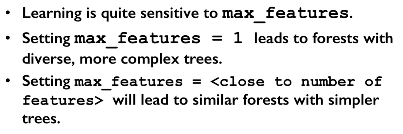This process is repeated to generate n samples, using the parameter n_estimators, which will eventually generate n number decision trees.
• Splitting Features: When picking the best split for a node, instead of finding the best split across all possible features (decision tree), a random subset of features is chosen and the best split is found within that smaller subset of features. The number of features in the subset that are randomly considered at each stage is controlled by the max_features parameter.

This randomness in selecting the bootstrap sample to train an individual tree in a forest ensemble, combined with the fact that splitting a node in the tree is restricted to random subsets of the features of the split, virtually guarantees that all of the decision trees and the random forest will be different.

University of Michigan: Coursera Data Science in Python

Prediction is then averaged among the trees.

University of Michigan: Coursera Data Science in Python

Key parameters include n_estimators, max_features, max_depth, n_jobs.

###### IMPORT MODULES #### ###
import pandas as pd
import numpy as np
from sklearn.ensemble import RandomForestClassifier
from sklearn.cross_validation import train_test_split
import sklearn.metrics



#### TRAIN TEST SPLIT ####
train_feature, test_feature, train_target, test_target = \
train_test_split(feature, target, test_size=0.2)

print train_feature.shape
print test_feature.shape
(404, 13)
(102, 13)


#### CREATE MODEL ####
# use 100 decision trees
clf = RandomForestClassifier(n_estimators=100, n_jobs=4, verbose=3)



#### FIT MODEL ####
model = clf.fit(train_feature, train_target)
print model
RandomForestClassifier(bootstrap=True, class_weight=None, criterion='gini',
            max_depth=None, max_features='auto', max_leaf_nodes=None,
            min_samples_leaf=1, min_samples_split=2,
            min_weight_fraction_leaf=0.0, n_estimators=100, n_jobs=1,
            oob_score=False, random_state=None, verbose=0,
            warm_start=False)



#### TEST MODEL ####
predictions = model.predict(test_feature)



#### SCORE MODEL ####
print 'accuracy', '\n', sklearn.metrics.accuracy_score(test_target, predictions)*100, '%', '\n'
print 'confusion matrix', '\n', sklearn.metrics.confusion_matrix(test_target,predictions)
accuracy
82.3529411765 %
confusion matrix
[[21  0  3]
 [ 0 21  4]
 [ 8  3 42]]



####### FEATURE IMPORTANCE #### ####
# rank the importance of features
f_impt= pd.DataFrame(model.feature_importances_, index=df.columns[:-2])
f_impt = f_impt.sort_values(by=0,ascending=False)
f_impt.columns = ['feature importance']

RM    0.225612
LSTAT 0.192478
CRIM  0.108510
DIS   0.088056
AGE   0.074202
NOX   0.067718
B     0.057706
PTRATIO       0.051702
TAX   0.047568
INDUS 0.037871
RAD   0.026538
ZN    0.012635
CHAS  0.009405



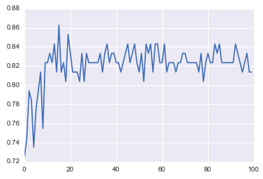
#### GRAPHS ####

# see how many decision trees are minimally required make the accuarcy consistent
import numpy as np
import matplotlib.pylab as plt
import seaborn as sns
%matplotlib inline

trees=range(100)
accuracy=np.zeros(100)

for i in range(len(trees)):
  clf=RandomForestClassifier(n_estimators= i+1)
  model=clf.fit(train_feature, train_target)
  predictions=model.predict(test_feature)
  accuracy[i]=sklearn.metrics.accuracy_score(test_target, predictions)

plt.plot(trees,accuracy)

# well, seems like more than 10 trees will have a consistent accuracy of 0.82.
# Guess there's no need to have an ensemble of 100 trees!

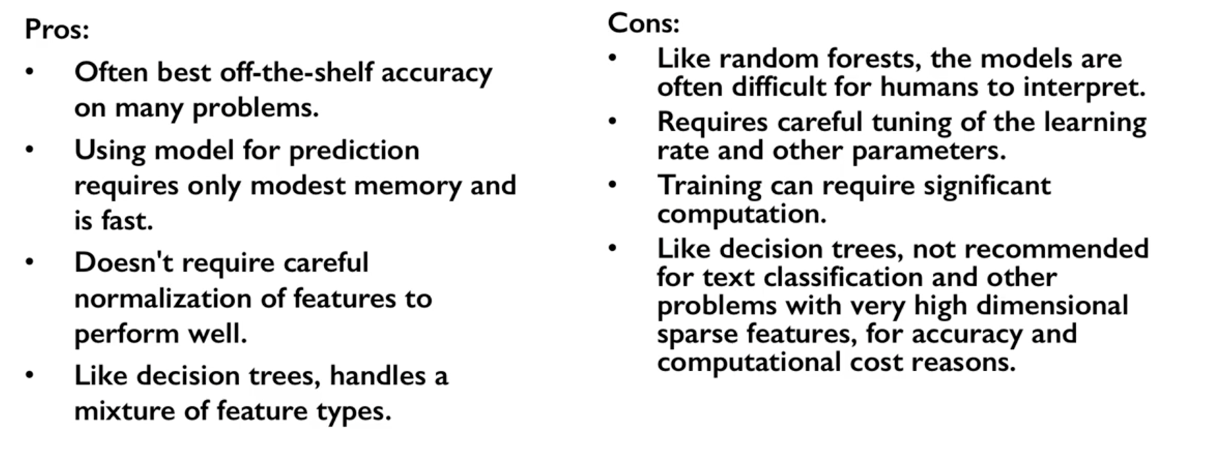
9.1.5. Gradient Boosted Decision Trees

Gradient Boosted Decision Trees (GBDT) builds a series of small decision trees, with each tree attempting to correct errors from previous stage. Here’s a good video on it, which describes AdaBoost, but gives a good overview of tree boosting models.

Typically, gradient boosted tree ensembles use lots of shallow trees known in machine learning as weak learners. Built in a nonrandom way, to create a model that makes fewer and fewer mistakes as more trees are added. Once the model is built, making predictions with a gradient boosted tree models is fast and doesn’t use a lot of memory.

learning_rate parameter controls how hard each tree tries to correct mistakes from previous round. High learning rate, more complex trees.

Key parameters, n_estimators, learning_rate, max_depth.

University of Michigan: Coursera Data Science in Python

from sklearn.ensemble import GradientBoostingClassifier

X_train, X_test, y_train, y_test = train_test_split(X_cancer, y_cancer, random_state = 0)


# Default Parameters
clf = GradientBoostingClassifier(random_state = 0)
clf.fit(X_train, y_train)

print('Breast cancer dataset (learning_rate=0.1, max_depth=3)')
print('Accuracy of GBDT classifier on training set: {:.2f}'
     .format(clf.score(X_train, y_train)))
print('Accuracy of GBDT classifier on test set: {:.2f}\n'
     .format(clf.score(X_test, y_test)))

# Adjusting Learning Rate & Max Depth
clf = GradientBoostingClassifier(learning_rate = 0.01, max_depth = 2, random_state = 0)
clf.fit(X_train, y_train)

print('Breast cancer dataset (learning_rate=0.01, max_depth=2)')
print('Accuracy of GBDT classifier on training set: {:.2f}'
     .format(clf.score(X_train, y_train)))
print('Accuracy of GBDT classifier on test set: {:.2f}'
     .format(clf.score(X_test, y_test)))


# Results
Breast cancer dataset (learning_rate=0.1, max_depth=3)
Accuracy of GBDT classifier on training set: 1.00
Accuracy of GBDT classifier on test set: 0.96

Breast cancer dataset (learning_rate=0.01, max_depth=2)
Accuracy of GBDT classifier on training set: 0.97
Accuracy of GBDT classifier on test set: 0.97

9.1.6. XGBoost

XGBoost or eXtreme Gradient Boosting, is a form of gradient boosted decision trees is that designed to be highly efficient, flexible and portable. It is one of the highly dominative classifier in competitive machine learning competitions.

https://www.analyticsvidhya.com/blog/2016/03/complete-guide-parameter-tuning-xgboost-with-codes-python/#

from xgboost import XGBClassifier
from sklearn.model_selection import train_test_split
from sklearn.metrics import accuracy_score

X_train, X_test, y_train, y_test = train_test_split(X, Y, random_state=0)

# fit model no training data
model = XGBClassifier()
model.fit(X_train, y_train)

# make predictions for test data
y_pred = model.predict(X_test)
predictions = [round(value) for value in y_pred]

# evaluate predictions
accuracy = accuracy_score(y_test, predictions)
print("Accuracy: %.2f%%" % (accuracy * 100.0))

9.1.7. LightGBM

LightGBM (Light Gradient Boosting) is a lightweight version of gradient boosting developed by Microsoft. It has similar performance to XGBoost but can run much faster than it.

https://lightgbm.readthedocs.io/en/latest/index.html

import lightgbm

X_train, X_test, y_train, y_test = train_test_split(x, y, test_size=0.2, random_state=42, stratify=y)

# Create the LightGBM data containers
train_data = lightgbm.Dataset(X_train, label=y)
test_data = lightgbm.Dataset(X_test, label=y_test)

parameters = {
  'application': 'binary',
  'objective': 'binary',
  'metric': 'auc',
  'is_unbalance': 'true',
  'boosting': 'gbdt',
  'num_leaves': 31,
  'feature_fraction': 0.5,
  'bagging_fraction': 0.5,
  'bagging_freq': 20,
  'learning_rate': 0.05,
  'verbose': 0
}

model = lightgbm.train(parameters,
                      train_data,
                      valid_sets=test_data,
                      num_boost_round=5000,
                      early_stopping_rounds=100)

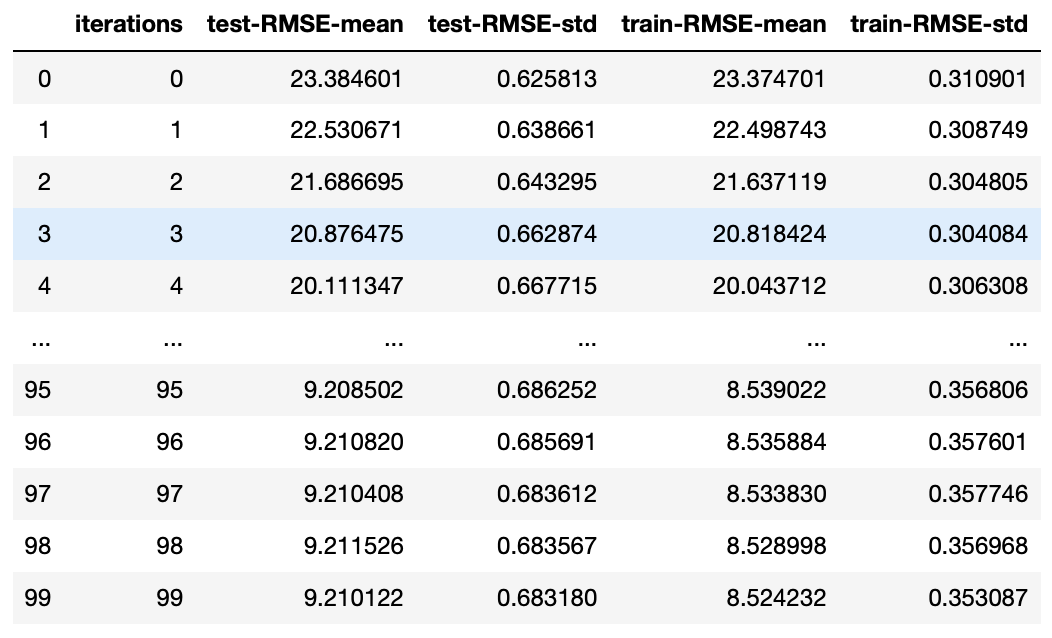
9.1.8. CatBoost

Category Boosting has high performance compared to other popular models, and does not require conversion of categorical values into numbers. It is said to be even faster than LighGBM, and allows model to be ran using GPU. For easy use, run in Colab & switch runtime to GPU.

More:

• https://catboost.ai
• https://github.com/catboost/tutorials/blob/master/classification/classification_tutorial.ipynb

from catboost import CatBoostRegressor

# Split dataset into
train_pool = Pool(train_X, train_y,
                  cat_features=['col1','col2'])
test_pool = Pool(test_X, test_y,
                 cat_features=['col1','col2'])

# Set Model Parameters
model = catboost.CatBoostRegressor(iterations=1000,
                                   learning_rate=0.1,
                                   loss_function='RMSE',
                                   early_stopping_rounds=5)

# Model Fitting
# verbose, gives output every n iteration
model.fit(X_train, y_train,
          cat_features=cat_features,
          eval_set=(X_test, y_test),
          verbose=5,
          task_type='GPU')

# Get Parameters
model.get_all_params

# Prediction, & Prediction Probabilities
predict = model.predict(data=X_test)
predict_prob = model.predict_proba(data=X_test)

# Evaluation
model.get_feature_importance(prettified=True)

We can also use k-fold cross validation for better scoring evaluation. There is no need to specify CatBoostRegressor or CatBoostClassifier, just input the correct eval_metric. One of the folds will be used as a validation set.

More: https://catboost.ai/docs/concepts/python-reference_cv.html

params = {"iterations": 100,
          "learning_rate": 0.05,
          "eval_metric": "RMSE",
          "verbose": False} # Default Parameters

cat_feat = [] # Categorical features list
cv_dataset = cgb.Pool(data=X, label=y, cat_features=cat_feat)

# CV scores
scores = catboost.cv(cv_dataset, params, fold_count=5)
scores

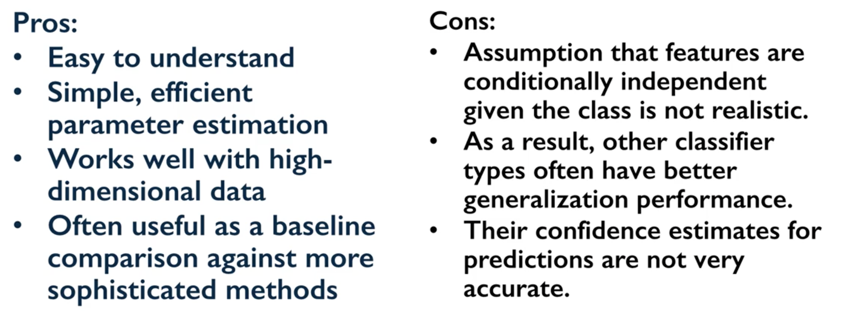
9.1.9. Naive Bayes

Naive Bayes is a probabilistic model. Features are assumed to be independent of each other in a given class. This makes the math very easy. E.g., words that are unrelated multiply together to form the final probability.

Prior Probability: Pr(y). Probability that a class (y) occurred in entire training dataset

Liklihood: Pr(y|xi) Probability of a class (y) occuring given all the features (xi).

There are 3 types of Naive Bayes:

• Bernouli: binary features (absence/presence of words)
• Multinomial: discrete features (account for frequency of words too, TF-IDF [frequency–inverse document frequency])
• Gaussian: continuous / real-value features (stores aerage avlue & standard deviation of each feature for each class)

Bernouli and Multinomial models are commonly used for sparse count data like text classification. The latter normally works better. Gaussian model is used for high-dimensional data.

University of Michigan: Coursera Data Science in Python

Sklearn allows partial fitting, i.e., fit the model incrementally if dataset is too large for memory.

Naive Bayes model only have one smoothing parameter called alpha (default 0.1). It adds a virtual data point that have positive values for all features. This is necessary considering that if there are no positive feature, the entire probability will be 0 (since it is a multiplicative model). More alpha means more smoothing, and more generalisation (less complex) model.

from sklearn.naive_bayes import GaussianNB
from adspy_shared_utilities import plot_class_regions_for_classifier

X_train, X_test, y_train, y_test = train_test_split(X_C2, y_C2, random_state=0)

# no parameters for tuning
nbclf = GaussianNB().fit(X_train, y_train)
plot_class_regions_for_classifier(nbclf, X_train, y_train, X_test, y_test,
                               'Gaussian Naive Bayes classifier: Dataset 1')

print('Accuracy of GaussianNB classifier on training set: {:.2f}'
    .format(nbclf.score(X_train, y_train)))
print('Accuracy of GaussianNB classifier on test set: {:.2f}'
    .format(nbclf.score(X_test, y_test)))

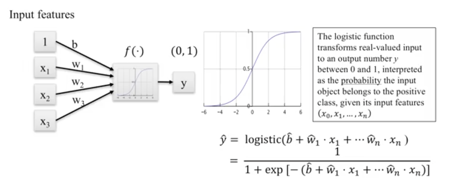
9.1.10. Logistic Regression

Binary output or y value. Functions are available in both statsmodels and sklearn packages.

#### IMPORT MODULES ####
import pandas as pd
import statsmodels.api as sm



#### FIT MODEL ####
lreg = sm.Logit(df3['diameter_cut'], df3[trainC]).fit()
print lreg.summary()



Optimization terminated successfully.
       Current function value: 0.518121
       Iterations 6
                           Logit Regression Results
==============================================================================
Dep. Variable:           diameter_cut   No. Observations:                18067
Model:                          Logit   Df Residuals:                    18065
Method:                           MLE   Df Model:                            1
Date:                Thu, 04 Aug 2016   Pseudo R-squ.:                  0.2525
Time:                        14:13:14   Log-Likelihood:                -9360.9
converged:                       True   LL-Null:                       -12523.
                                        LLR p-value:                     0.000
================================================================================
                   coef    std err          z      P>|z|      [95.0% Conf. Int.]
--------------------------------------------------------------------------------
depth            4.2529      0.067     63.250      0.000         4.121     4.385
layers_YESNO    -2.1102      0.037    -57.679      0.000        -2.182    -2.039
================================================================================



#### CONFIDENCE INTERVALS ####
params = lreg.params
conf = lreg.conf_int()
conf['OR'] = params
conf.columns = ['Lower CI', 'Upper CI', 'OR']
print (np.exp(conf))

Lower CI   Upper CI         OR
depth         61.625434  80.209893  70.306255
layers_YESNO   0.112824   0.130223   0.121212

A regularisation penlty L2, just like ridge regression is by default in sklearn.linear_model, LogisticRegression, controlled using the parameter C (default 1).

from sklearn.linear_model import LogisticRegression
from adspy_shared_utilities import (plot_class_regions_for_classifier_subplot)

fig, subaxes = plt.subplots(1, 1, figsize=(7, 5))
y_fruits_apple = y_fruits_2d == 1   # make into a binary problem: apples vs everything else
X_train, X_test, y_train, y_test = (
train_test_split(X_fruits_2d.as_matrix(),
                y_fruits_apple.as_matrix(),
                random_state = 0))

clf = LogisticRegression(C=100).fit(X_train, y_train)
plot_class_regions_for_classifier_subplot(clf, X_train, y_train, None,
                                         None, 'Logistic regression \
for binary classification\nFruit dataset: Apple vs others',
                                         subaxes)

h = 6
w = 8
print('A fruit with height {} and width {} is predicted to be: {}'
     .format(h,w, ['not an apple', 'an apple'][clf.predict([[h,w]])[0]]))

h = 10
w = 7
print('A fruit with height {} and width {} is predicted to be: {}'
     .format(h,w, ['not an apple', 'an apple'][clf.predict([[h,w]])[0]]))
subaxes.set_xlabel('height')
subaxes.set_ylabel('width')

print('Accuracy of Logistic regression classifier on training set: {:.2f}'
     .format(clf.score(X_train, y_train)))
print('Accuracy of Logistic regression classifier on test set: {:.2f}'
     .format(clf.score(X_test, y_test)))

9.1.11. Support Vector Machine

Support Vector Machines (SVM) involves locating the support vectors of two boundaries to find a maximum tolerance hyperplane. Side note: linear kernels work best for text classification.

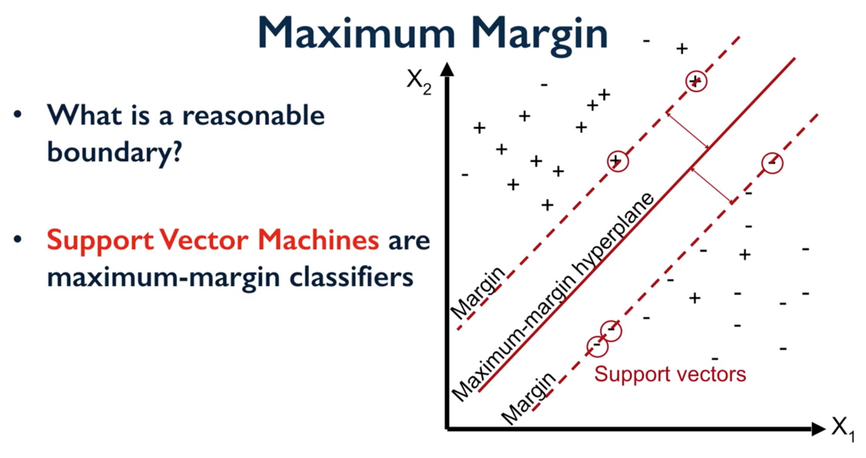
University of Michigan: Coursera Data Science in Python

Have 3 tuning parameters. Need to normalize first too!

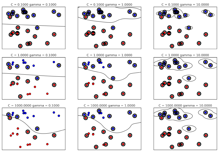
1. Have regularisation using parameter C, just like logistic regression. Default to 1. Limits the importance of each point.
2. Type of kernel. Default is Radial Basis Function (RBF)
3. Gamma parameter for adjusting kernel width. Influence of a single training example reaches. Low gamma > far reach, high values > limited reach.

from sklearn.svm import SVC
from adspy_shared_utilities import plot_class_regions_for_classifier_subplot


X_train, X_test, y_train, y_test = train_test_split(X_C2, y_C2, random_state = 0)

fig, subaxes = plt.subplots(1, 1, figsize=(7, 5))
this_C = 1.0
clf = SVC(kernel = 'linear', C=this_C).fit(X_train, y_train)
title = 'Linear SVC, C = {:.3f}'.format(this_C)
plot_class_regions_for_classifier_subplot(clf, X_train, y_train, None, None, title, subaxes)

We can directly call a linear SVC by directly importing the LinearSVC function

from sklearn.svm import LinearSVC
X_train, X_test, y_train, y_test = train_test_split(X_cancer, y_cancer, random_state = 0)

clf = LinearSVC().fit(X_train, y_train)
print('Breast cancer dataset')
print('Accuracy of Linear SVC classifier on training set: {:.2f}'
     .format(clf.score(X_train, y_train)))
print('Accuracy of Linear SVC classifier on test set: {:.2f}'
     .format(clf.score(X_test, y_test)))

Multi-Class Classification, i.e., having more than 2 target values, is also possible. With the results, it is possible to compare one class versus all other classes.

from sklearn.svm import LinearSVC

X_train, X_test, y_train, y_test = train_test_split(X_fruits_2d, y_fruits_2d, random_state = 0)

clf = LinearSVC(C=5, random_state = 67).fit(X_train, y_train)
print('Coefficients:\n', clf.coef_)
print('Intercepts:\n', clf.intercept_)

visualising in a graph…

plt.figure(figsize=(6,6))
colors = ['r', 'g', 'b', 'y']
cmap_fruits = ListedColormap(['#FF0000', '#00FF00', '#0000FF','#FFFF00'])

plt.scatter(X_fruits_2d[['height']], X_fruits_2d[['width']],
           c=y_fruits_2d, cmap=cmap_fruits, edgecolor = 'black', alpha=.7)

x_0_range = np.linspace(-10, 15)

for w, b, color in zip(clf.coef_, clf.intercept_, ['r', 'g', 'b', 'y']):
    # Since class prediction with a linear model uses the formula y = w_0 x_0 + w_1 x_1 + b,
    # and the decision boundary is defined as being all points with y = 0, to plot x_1 as a
    # function of x_0 we just solve w_0 x_0 + w_1 x_1 + b = 0 for x_1:
    plt.plot(x_0_range, -(x_0_range * w[0] + b) / w[1], c=color, alpha=.8)

plt.legend(target_names_fruits)
plt.xlabel('height')
plt.ylabel('width')
plt.xlim(-2, 12)
plt.ylim(-2, 15)
plt.show()

Kernalised Support Vector Machines

For complex classification, new dimensions can be added to SVM. e.g., square of x. There are many types of kernal transformations. By default, SVM will use the Radial Basis Function (RBF) kernel.

from sklearn.svm import SVC
from adspy_shared_utilities import plot_class_regions_for_classifier

X_train, X_test, y_train, y_test = train_test_split(X_D2, y_D2, random_state = 0)

# The default SVC kernel is radial basis function (RBF)
plot_class_regions_for_classifier(SVC().fit(X_train, y_train),
                                 X_train, y_train, None, None,
                                 'Support Vector Classifier: RBF kernel')

# Compare decision boundries with polynomial kernel, degree = 3
plot_class_regions_for_classifier(SVC(kernel = 'poly', degree = 3)
                                 .fit(X_train, y_train), X_train,
                                 y_train, None, None,
                                 'Support Vector Classifier: Polynomial kernel, degree = 3')

Full tuning in Support Vector Machines, using normalisation, kernel tuning, and regularisation.

from sklearn.preprocessing import MinMaxScaler
scaler = MinMaxScaler()
X_train_scaled = scaler.fit_transform(X_train)
X_test_scaled = scaler.transform(X_test)

clf = SVC(kernel = 'rbf', gamma=1, C=10).fit(X_train_scaled, y_train)
print('Breast cancer dataset (normalized with MinMax scaling)')
print('RBF-kernel SVC (with MinMax scaling) training set accuracy: {:.2f}'
     .format(clf.score(X_train_scaled, y_train)))
print('RBF-kernel SVC (with MinMax scaling) test set accuracy: {:.2f}'
     .format(clf.score(X_test_scaled, y_test)))

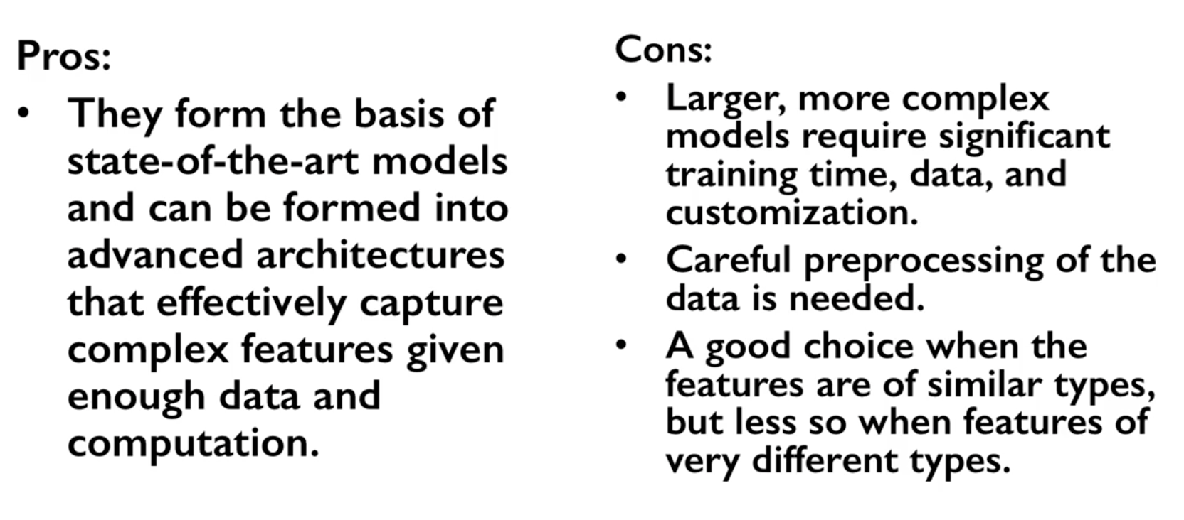
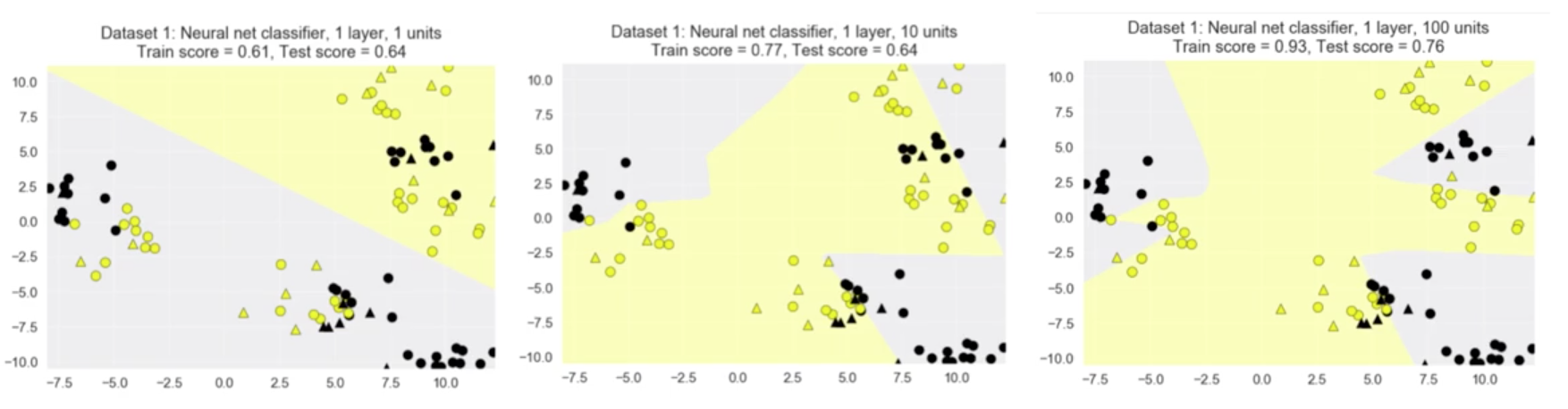
9.1.12. Neural Networks

Examples using Multi-Layer Perceptrons (MLP).

University of Michigan: Coursera Data Science in Python

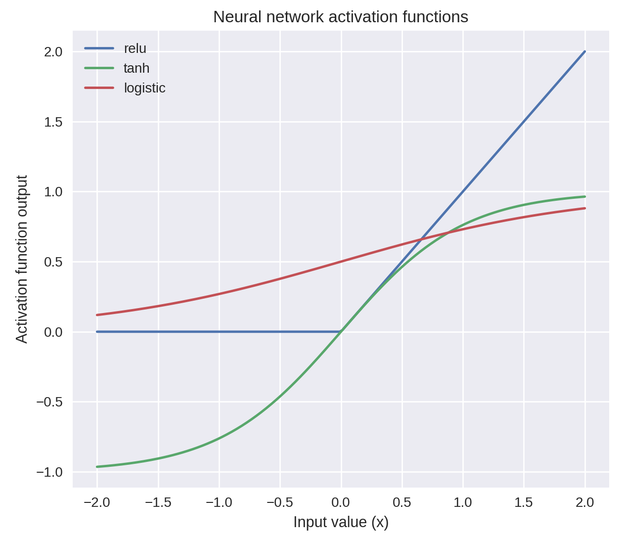
Activation Function. University of Michigan: Coursera Data Science in Python

Parameters include

• hidden_layer_sizes which is the number of hidden layers, with no. units in each layer (default 100).
• solvers is the algorithm usedthat does the numerical work of finding the optimal weights. default adam used for large datasets, lbfgs is used for smaller datasets.
• alpha: L2 regularisation, default is 0.0001,
• activation: non-linear function used for activation function which include relu (default), logistic, tanh

One Hidden Layer

from sklearn.neural_network import MLPClassifier
from adspy_shared_utilities import plot_class_regions_for_classifier_subplot

X_train, X_test, y_train, y_test = train_test_split(X_D2, y_D2, random_state=0)

fig, subaxes = plt.subplots(3, 1, figsize=(6,18))


for units, axis in zip([1, 10, 100], subaxes):
    nnclf = MLPClassifier(hidden_layer_sizes = [units], solver='lbfgs',
                         random_state = 0).fit(X_train, y_train)

    title = 'Dataset 1: Neural net classifier, 1 layer, {} units'.format(units)

    plot_class_regions_for_classifier_subplot(nnclf, X_train, y_train,
                                             X_test, y_test, title, axis)
    plt.tight_layout()

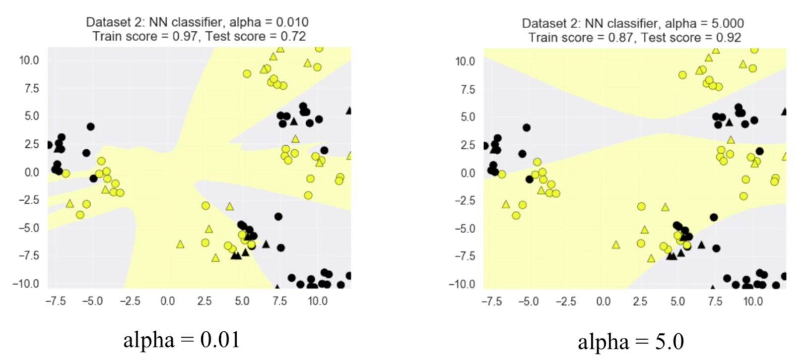
Two Hidden Layers, L2 Regularisation (alpha), Activation

X_train, X_test, y_train, y_test = train_test_split(X_D2, y_D2, random_state=0)

fig, subaxes = plt.subplots(4, 1, figsize=(6, 23))

for this_alpha, axis in zip([0.01, 0.1, 1.0, 5.0], subaxes):
    nnclf = MLPClassifier(solver='lbfgs', activation = 'tanh',
                         alpha = this_alpha,
                         hidden_layer_sizes = [100, 100],
                         random_state = 0).fit(X_train, y_train)

    title = 'Dataset 2: NN classifier, alpha = {:.3f} '.format(this_alpha)

    plot_class_regions_for_classifier_subplot(nnclf, X_train, y_train,
                                             X_test, y_test, title, axis)
    plt.tight_layout()

Normalisation: Input features should be normalised.

from sklearn.neural_network import MLPClassifier
from sklearn.preprocessing import MinMaxScaler


scaler = MinMaxScaler()

X_train, X_test, y_train, y_test = train_test_split(X_cancer, y_cancer, random_state = 0)
X_train_scaled = scaler.fit_transform(X_train)
X_test_scaled = scaler.transform(X_test)

clf = MLPClassifier(hidden_layer_sizes = [100, 100], alpha = 5.0,
                   random_state = 0, solver='lbfgs').fit(X_train_scaled, y_train)

print('Breast cancer dataset')
print('Accuracy of NN classifier on training set: {:.2f}'
     .format(clf.score(X_train_scaled, y_train)))
print('Accuracy of NN classifier on test set: {:.2f}'
     .format(clf.score(X_test_scaled, y_test)))


# RESULTS
Breast cancer dataset
Accuracy of NN classifier on training set: 0.98
Accuracy of NN classifier on test set: 0.97

9.2. Regression

When response is a continuous value.

9.2.1. OLS Regression

Ordinary Least Squares Regression or OLS Regression is the most basic form and fundamental of regression. Best fit line ŷ = a + bx is drawn based on the ordinary least squares method. i.e., least total area of squares (sum of squares) with length from each x,y point to regresson line.

OLS can be conducted using statsmodel package.

model = smf.ols(formula='diameter ~ depth', data=df3).fit()
print model.summary()



OLS Regression Results
==============================================================================
Dep. Variable:               diameter   R-squared:                       0.512
Model:                            OLS   Adj. R-squared:                  0.512
Method:                 Least Squares   F-statistic:                 1.895e+04
Date:                Tue, 02 Aug 2016   Prob (F-statistic):               0.00
Time:                        17:10:34   Log-Likelihood:                -51812.
No. Observations:               18067   AIC:                         1.036e+05
Df Residuals:                   18065   BIC:                         1.036e+05
Df Model:                           1
Covariance Type:            nonrobust
==============================================================================
coef    std err          t      P>|t|      [95.0% Conf. Int.]
------------------------------------------------------------------------------
Intercept      2.2523      0.054     41.656      0.000         2.146     2.358
depth         11.5836      0.084    137.675      0.000        11.419    11.749
==============================================================================
Omnibus:                    12117.030   Durbin-Watson:                   0.673
Prob(Omnibus):                  0.000   Jarque-Bera (JB):           391356.565
Skew:                           2.771   Prob(JB):                         0.00
Kurtosis:                      25.117   Cond. No.                         3.46
==============================================================================

Warnings:
[1] Standard Errors assume that the covariance matrix of the errors is correctly specified.

or sci-kit learn package

from sklearn import linear_model

reg = linear_model.LinearRegression()
model = reg.fit ([[0, 0], [1, 1], [2, 2]], [0, 1, 2])

model
LinearRegression(copy_X=True, fit_intercept=True, n_jobs=1, normalize=False)
reg.coef_
array([ 0.5,  0.5])

# R2 scores
r2_trains = model.score(X_train, y_train)
r2_tests = model.score(X_test, y_test)

9.2.2. Ridge Regression

Regularisaton is an important concept used in Ridge Regression as well as the next LASSO regression. Ridge regression uses regularisation which adds a penalty parameter to a variable when it has a large variation. Regularisation prevents overfitting by restricting the model, thus lowering its complexity.

• Uses L2 regularisation, which reduces the sum of squares of the parameters
• The influence of L2 is controlled by an alpha parameter. Default is 1.
• High alpha means more regularisation and a simpler model.
• More in https://www.analyticsvidhya.com/blog/2016/01/complete-tutorial-ridge-lasso-regression-python/

#### IMPORT MODULES ####
import panda as pd
import numpy as np
from sklearn.linear_model import Ridge
from sklearn.preprocessing import MinMaxScaler

#### TRAIN-TEST SPLIT ####
X_train, X_test, y_train, y_test = train_test_split(X_crime, y_crime,
                                                 random_state = 0)

#### NORMALIZATION ####
  # using minmaxscaler
scaler = MinMaxScaler()
X_train_scaled = scaler.fit_transform(X_train)
X_test_scaled = scaler.transform(X_test)


#### CREATE AND FIT MODEL ####
linridge = Ridge(alpha=20.0).fit(X_train_scaled, y_train)

print('Crime dataset')
print('ridge regression linear model intercept: {}'
   .format(linridge.intercept_))
print('ridge regression linear model coeff:\n{}'
   .format(linridge.coef_))
print('R-squared score (training): {:.3f}'
   .format(linridge.score(X_train_scaled, y_train)))
print('R-squared score (test): {:.3f}'
   .format(linridge.score(X_test_scaled, y_test)))
print('Number of non-zero features: {}'
   .format(np.sum(linridge.coef_ != 0)))

To investigate the effect of alpha:

print('Ridge regression: effect of alpha regularization parameter\n')
for this_alpha in [0, 1, 10, 20, 50, 100, 1000]:
  linridge = Ridge(alpha = this_alpha).fit(X_train_scaled, y_train)
  r2_train = linridge.score(X_train_scaled, y_train)
  r2_test = linridge.score(X_test_scaled, y_test)
  num_coeff_bigger = np.sum(abs(linridge.coef_) > 1.0)
  print('Alpha = {:.2f}\nnum abs(coeff) > 1.0: {}, \
        r-squared training: {:.2f}, r-squared test: {:.2f}\n'
       .format(this_alpha, num_coeff_bigger, r2_train, r2_test))

Note

• Many variables with small/medium effects: Ridge
• Only a few variables with medium/large effects: LASSO

9.2.3. LASSO Regression

LASSO refers to Least Absolute Shrinkage and Selection Operator Regression. Like Ridge Regression this also has a regularisation property.

• Uses L1 regularisation, which reduces sum of the absolute values of coefficients, that change unimportant features (their regression coefficients) into 0
• This is known as a sparse solution, or a kind of feature selection, since some variables were removed in the process
• The influence of L1 is controlled by an alpha parameter. Default is 1.
• High alpha means more regularisation and a simpler model. When alpha = 0, then it is a normal OLS regression.

1. Bias increase & variability decreases when alpha increases.
2. Useful when there are many features (explanatory variables).
3. Have to standardize all features so that they have mean 0 and std error 1.
4. Have several algorithms: LAR (Least Angle Regression). Starts w 0 predictors & add each predictor that is most correlated at each step.

#### IMPORT MODULES ####
import pandas as pd
import numpy as py
from sklearn import preprocessing
from sklearn.cross_validation import train_test_split
from sklearn.linear_model import LassoLarsCV
import sklearn.metrics
from sklearn.datasets import load_boston



#### NORMALIZATION ####
# standardise the means to 0 and standard error to 1
for i in df.columns[:-1]: # df.columns[:-1] = dataframe for all features
  df[i] = preprocessing.scale(df[i].astype('float64'))
df.describe()



#### TRAIN TEST SPLIT ####
train_feature, test_feature, train_target, test_target = \
train_test_split(feature, target, random_state=123, test_size=0.2)

print train_feature.shape
print test_feature.shape
(404, 13)
(102, 13)



#### CREATE MODEL ####
# Fit the LASSO LAR regression model
# cv=10; use k-fold cross validation
# precompute; True=model will be faster if dataset is large
model=LassoLarsCV(cv=10, precompute=False)



#### FIT MODEL ####
model = model.fit(train_feature,train_target)
print model
LassoLarsCV(copy_X=True, cv=10, eps=2.2204460492503131e-16,
      fit_intercept=True, max_iter=500, max_n_alphas=1000, n_jobs=1,
      normalize=True, positive=False, precompute=False, verbose=False)



#### ANALYSE COEFFICIENTS ####
Compare the regression coefficients, and see which one LASSO removed.
LSTAT is the most important predictor, followed by RM, DIS, and RAD. AGE is removed by LASSO

df2=pd.DataFrame(model.coef_, index=feature.columns)
df2.sort_values(by=0,ascending=False)
RM    3.050843
RAD   2.040252
ZN    1.004318
B     0.629933
CHAS  0.317948
INDUS 0.225688
AGE   0.000000
CRIM  -0.770291
NOX   -1.617137
TAX   -1.731576
PTRATIO       -1.923485
DIS   -2.733660
LSTAT -3.878356



#### SCORE MODEL ####
# MSE from training and test data
from sklearn.metrics import mean_squared_error
train_error = mean_squared_error(train_target, model.predict(train_feature))
test_error = mean_squared_error(test_target, model.predict(test_feature))

print ('training data MSE')
print(train_error)
print ('test data MSE')
print(test_error)

# MSE closer to 0 are better
# test dataset is less accurate as expected
training data MSE
20.7279948891
test data MSE
28.3767672242


# R-square from training and test data
rsquared_train=model.score(train_feature,train_target)
rsquared_test=model.score(test_feature,test_target)
print ('training data R-square')
print(rsquared_train)
print ('test data R-square')
print(rsquared_test)

# test data explained 65% of the predictors
training data R-square
0.755337444405
test data R-square
0.657019301268

9.2.4. Polynomial Regression

from sklearn.linear_model import LinearRegression
from sklearn.linear_model import Ridge
from sklearn.preprocessing import PolynomialFeatures


# Normal Linear Regression
X_train, X_test, y_train, y_test = train_test_split(X_F1, y_F1,
                                                   random_state = 0)
linreg = LinearRegression().fit(X_train, y_train)

print('linear model coeff (w): {}'
     .format(linreg.coef_))
print('linear model intercept (b): {:.3f}'
     .format(linreg.intercept_))
print('R-squared score (training): {:.3f}'
     .format(linreg.score(X_train, y_train)))
print('R-squared score (test): {:.3f}'
     .format(linreg.score(X_test, y_test)))

print('\nNow we transform the original input data to add\n\
polynomial features up to degree 2 (quadratic)\n')

# Polynomial Regression
poly = PolynomialFeatures(degree=2)
X_F1_poly = poly.fit_transform(X_F1)

X_train, X_test, y_train, y_test = train_test_split(X_F1_poly, y_F1,
                                                   random_state = 0)
linreg = LinearRegression().fit(X_train, y_train)

print('(poly deg 2) linear model coeff (w):\n{}'
     .format(linreg.coef_))
print('(poly deg 2) linear model intercept (b): {:.3f}'
     .format(linreg.intercept_))
print('(poly deg 2) R-squared score (training): {:.3f}'
     .format(linreg.score(X_train, y_train)))
print('(poly deg 2) R-squared score (test): {:.3f}\n'
     .format(linreg.score(X_test, y_test)))

# Polynomial with Ridge Regression
'''Addition of many polynomial features often leads to
overfitting, so we often use polynomial features in combination
with regression that has a regularization penalty, like ridge
regression.'''

X_train, X_test, y_train, y_test = train_test_split(X_F1_poly, y_F1,
                                                   random_state = 0)
linreg = Ridge().fit(X_train, y_train)

print('(poly deg 2 + ridge) linear model coeff (w):\n{}'
     .format(linreg.coef_))
print('(poly deg 2 + ridge) linear model intercept (b): {:.3f}'
     .format(linreg.intercept_))
print('(poly deg 2 + ridge) R-squared score (training): {:.3f}'
     .format(linreg.score(X_train, y_train)))
print('(poly deg 2 + ridge) R-squared score (test): {:.3f}'
     .format(linreg.score(X_test, y_test)))

9.2.5. Decision Tree Regressor

Same as decision tree classifier but the target is continuous.

from sklearn.tree import DecisionTreeRegressor

9.2.6. Random Forest Regressor

Same as randomforest classifier but the target is continuous.

from sklearn.ensemble import RandomForestRegressor

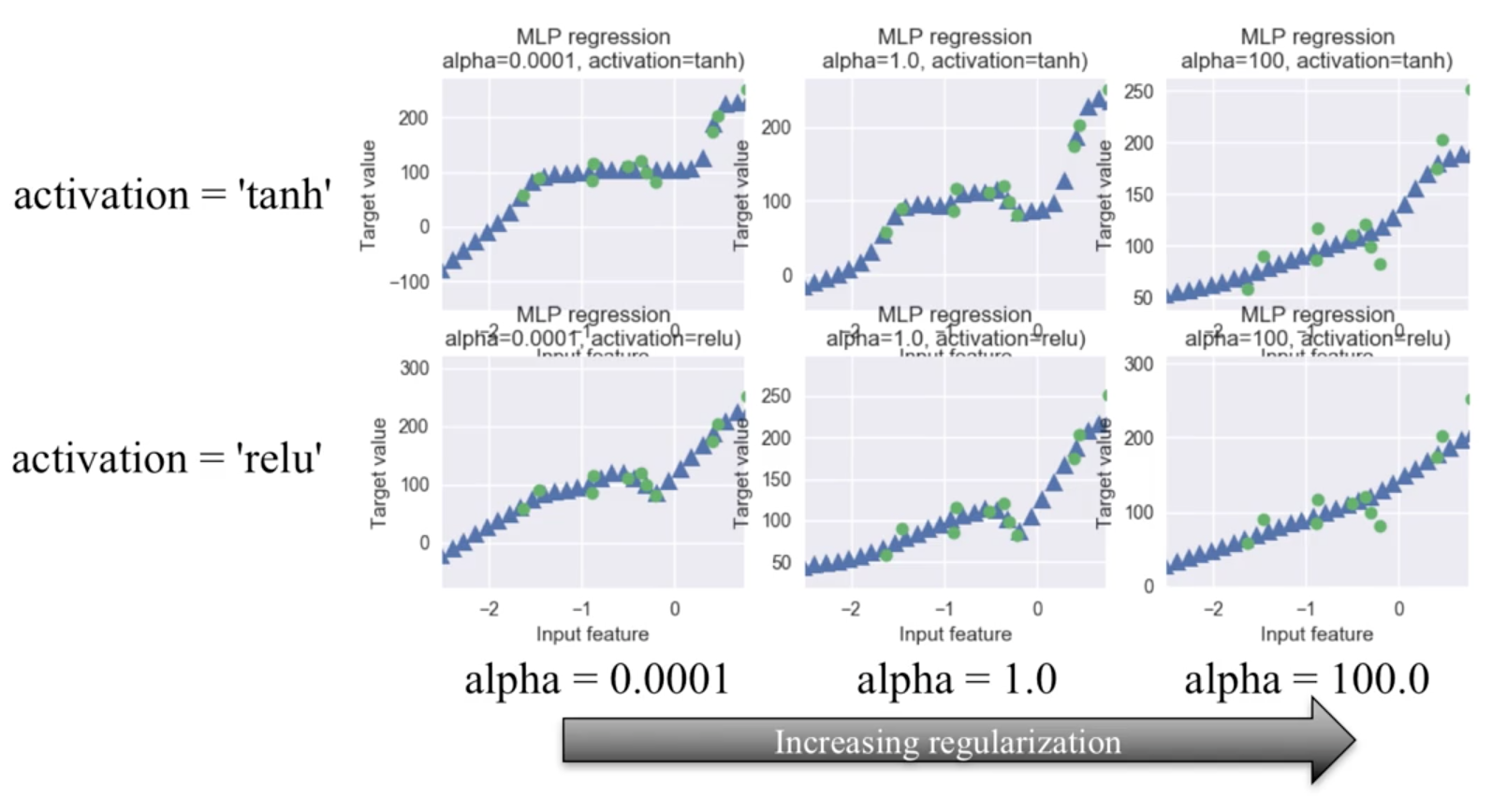
9.2.7. Neutral Networks

from sklearn.neural_network import MLPRegressor

fig, subaxes = plt.subplots(2, 3, figsize=(11,8), dpi=70)

X_predict_input = np.linspace(-3, 3, 50).reshape(-1,1)

X_train, X_test, y_train, y_test = train_test_split(X_R1[0::5], y_R1[0::5], random_state = 0)

for thisaxisrow, thisactivation in zip(subaxes, ['tanh', 'relu']):
    for thisalpha, thisaxis in zip([0.0001, 1.0, 100], thisaxisrow):
        mlpreg = MLPRegressor(hidden_layer_sizes = [100,100],
                             activation = thisactivation,
                             alpha = thisalpha,
                             solver = 'lbfgs').fit(X_train, y_train)
        y_predict_output = mlpreg.predict(X_predict_input)
        thisaxis.set_xlim([-2.5, 0.75])
        thisaxis.plot(X_predict_input, y_predict_output,
                     '^', markersize = 10)
        thisaxis.plot(X_train, y_train, 'o')
        thisaxis.set_xlabel('Input feature')
        thisaxis.set_ylabel('Target value')
        thisaxis.set_title('MLP regression\nalpha={}, activation={})'
                          .format(thisalpha, thisactivation))
        plt.tight_layout()