1. General Notes¶

1.1. Virtual Environment¶

Every project has a different set of requirements and different set of python packages to support it. The versions of each package can differ or break with each python or dependent packages update, so it is important to isolate every project within an enclosed virtual environment. Anaconda provides a straight forward way to manage this.

1.1.1. Creating the Virtual Env¶

# create environment, specify python base or it will copy all existing packages
conda create -n yourenvname anaconda
conda create -n yourenvname python=3.7
conda create -n yourenvname anaconda python=3.7

# activate environment
source activate yourenvname

# install package
conda install -n yourenvname [package]

# deactivate environment
conda deactivate

# delete environment
# -a = all, remove all packages in the environment
conda env remove -n yourenvname -a

# see all environments
conda env list

# create yml environment file
conda env export > environment.yml

An asterisk (*) will be placed at the current active environment.

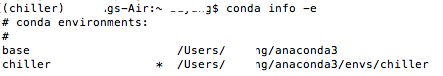
Current active environment

1.1.2. Using YMAL¶

Alternatively, we can create a fixed environment file and execute using conda env create -f environment.yml. This will create an environment with the name and packages specified within the folder. Channels specify where the packages are installed from.

name: environment_name
channels:
  - conda-forge
  - defaults
dependencies:
  - python=3.7
  - bokeh=0.9.2
  - numpy=1.9.*
  - pip:
    - baytune==0.3.1

1.1.3. Requirements.txt¶

If there is no ymal file specifying the packages to install, it is good practise to alternatively create a requirements.txt using the package pip install pipreqs. We can then create the txt in cmd using pipreqs -f directory_path, where -f overwrites any existing requirements.txt file.

Below is how the contents in a requirements.txt file looks like. After creating the file, and activating the VM, install the packages at one go using pip install -r requirements.txt.

pika==1.1.0
scipy==1.4.1
scikit_image==0.16.2
numpy==1.18.1
# package from github, not present in pip
git+https://github.com/cftang0827/pedestrian_detection_ssdlite
# wheel file stored in a website
--find-links https://dl.fbaipublicfiles.com/detectron2/wheels/cu101/index.html
detectron2
--find-links https://download.pytorch.org/whl/torch_stable.html
torch==1.5.0+cu101
torchvision==0.6.0+cu101

1.2. Modeling¶

A parsimonious model is a the model that accomplishes the desired level of prediction with as few predictor variables as possible.

1.2.1. Variables¶

x = independent variable = explanatory = predictor

y = dependent variable = response = target

1.2.2. Data Types¶

The type of data is essential as it determines what kind of tests can be applied to it.

Continuous: Also known as quantitative. Unlimited number of values

Categorical: Also known as discrete or qualitative. Fixed number of values or categories

1.2.3. Bias-Variance Tradeoff¶

The best predictive algorithm is one that has good Generalization Ability. With that, it will be able to give accurate predictions to new and previously unseen data.

High Bias results from Underfitting the model. This usually results from erroneous assumptions, and cause the model to be too general.

High Variance results from Overfitting the model, and it will predict the training dataset very accurately, but not with unseen new datasets. This is because it will fit even the slightless noise in the dataset.

The best model with the highest accuarcy is the middle ground between the two.

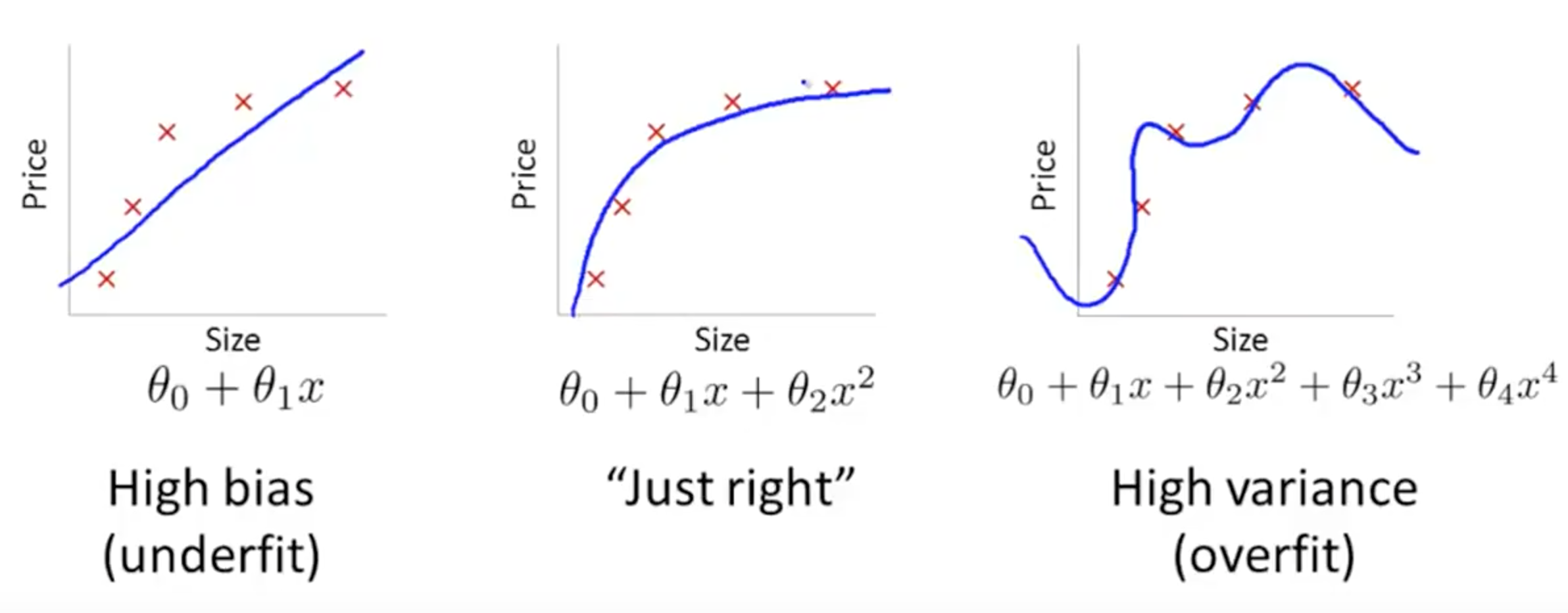
from Andrew Ng’s lecture

1.2.4. Steps to Build a Predictive Model¶

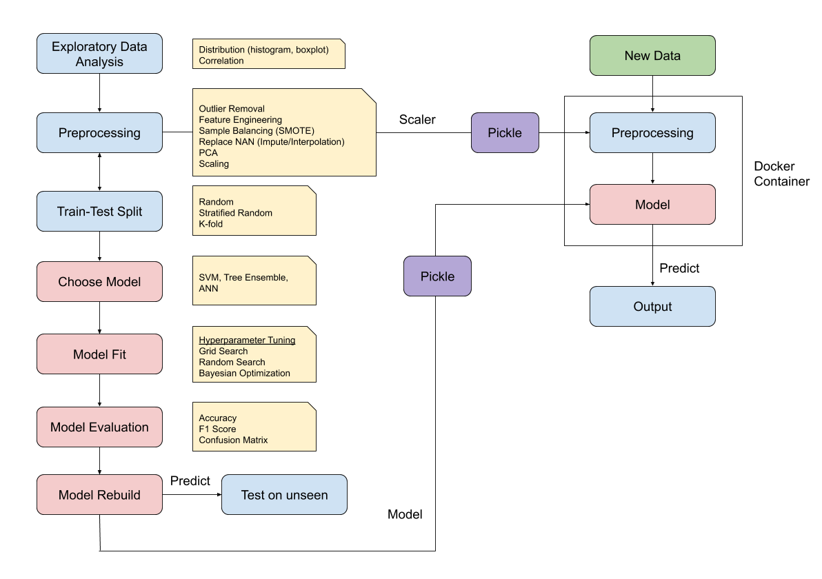
Typical architecture for model building for supervised classification

1.2.4.1. Feature Selection, Preprocessing, Extraction¶

Remove features that have too many NAN or fill NAN with another value

Remove features that will introduce data leakage

Encode categorical features into integers

Extract new useful features (between and within current features)

1.2.4.2. Normalise the Features¶

With the exception of Tree models and Naive Bayes, other machine learning techniques like Neural Networks, KNN, SVM should have their features scaled.

1.2.4.3. Train Test Split¶

Split the dataset into Train and Test datasets. By default, sklearn assigns 75% to train & 25% to test randomly. A random state (seed) can be selected to fixed the randomisation

from sklearn.model_selection import train_test_split

X_train, X_test, y_train, y_test
= train_test_split(predictor, target, test_size=0.25, random_state=0)

1.2.4.4. Create Model¶

Choose model and set model parameters (if any).

clf = DecisionTreeClassifier()

1.2.4.5. Fit Model¶

Fit the model using the training dataset.

model = clf.fit(X_train, y_train)

>>> print model
DecisionTreeClassifier(class_weight=None, criterion='gini', max_depth=None,
            max_features=None, max_leaf_nodes=None, min_samples_leaf=1,
            min_samples_split=2, min_weight_fraction_leaf=0.0,
            presort=False, random_state=None, splitter='best')

1.2.4.6. Test Model¶

Test the model by predicting identity of unseen data using the testing dataset.

y_predict = model.predict(X_test)

1.2.4.7. Score Model¶

Use a confusion matrix and…

>>> print sklearn.metrics.confusion_matrix(y_test, predictions)
[[14  0  0]
 [ 0 13  0]
 [ 0  1 10]]

accuarcy percentage, and f1 score to obtain the predictive accuarcy.

import sklearn.metrics
print sklearn.metrics.accuracy_score(y_test, y_predict)*100, '%'
>>> 97.3684210526 %

1.2.4.8. Cross Validation¶

When all code is working fine, remove the train-test portion and use Grid Search Cross Validation to compute the best parameters with cross validation.

1.2.4.9. Final Model¶

Finally, rebuild the model using the full dataset, and the chosen parameters tested.

1.2.5. Quick-Analysis for Multi-Models¶

import pandas as pd
from sklearn.preprocessing import StandardScaler
from sklearn.model_selection import train_test_split

from sklearn.svm import LinearSVC
from sklearn.svm import SVC
from sklearn.ensemble import RandomForestClassifier
from sklearn.ensemble import ExtraTreesClassifier
from xgboost import XGBClassifier

from sklearn.metrics import accuracy_score, f1_score
from statistics import mean
import seaborn as sns

# models to test
svml = LinearSVC()
svm = SVC()
rf = RandomForestClassifier()
xg = XGBClassifier()
xr = ExtraTreesClassifier()

# iterations
classifiers = [svml, svm, rf, xr, xg]
names = ['Linear SVM', 'RBF SVM', 'Random Forest', 'Extremely Randomized Trees', 'XGBoost']
results = []

# train-test split
X = df[df.columns[:-1]]
# normalise data for SVM
X = StandardScaler().fit(X).transform(X)
y = df['label']
X_train, X_test, y_train, y_test = train_test_split(X, y, random_state=0)

for name, clf in zip(names, classifiers):
    model = clf.fit(X_train, y_train)
    y_predict = model.predict(X_test)
    accuracy = accuracy_score(y_test, y_predict)
    f1 = mean(f1_score(y_test, y_predict, average=None))
    results.append([fault, name, accuracy, f1])

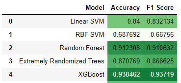
A final heatmap to compare the outcomes.

final = pd.DataFrame(results, columns=['Fault Type','Model','Accuracy','F1 Score'])
final.style.background_gradient(cmap='Greens')