13. Evaluation

Sklearn provides a good list of evaluation metrics for classification, regression and clustering problems.

http://scikit-learn.org/stable/modules/model_evaluation.html

In addition, it is also essential to know how to analyse the features and adjusting hyperparameters based on different evalution metrics.

13.1. Classification

13.1.1. Confusion Matrix

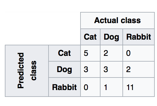
Wikipedia

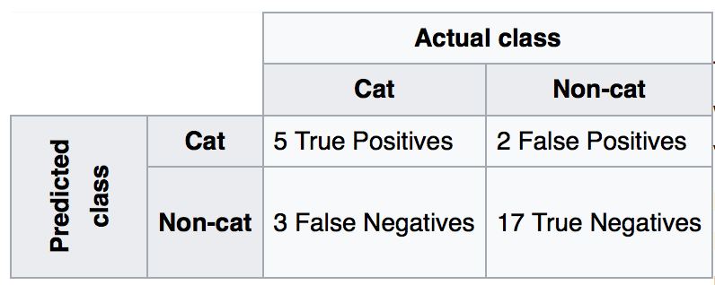
Wikipedia

https://www.youtube.com/watch?v=21Igj5Pr6u4

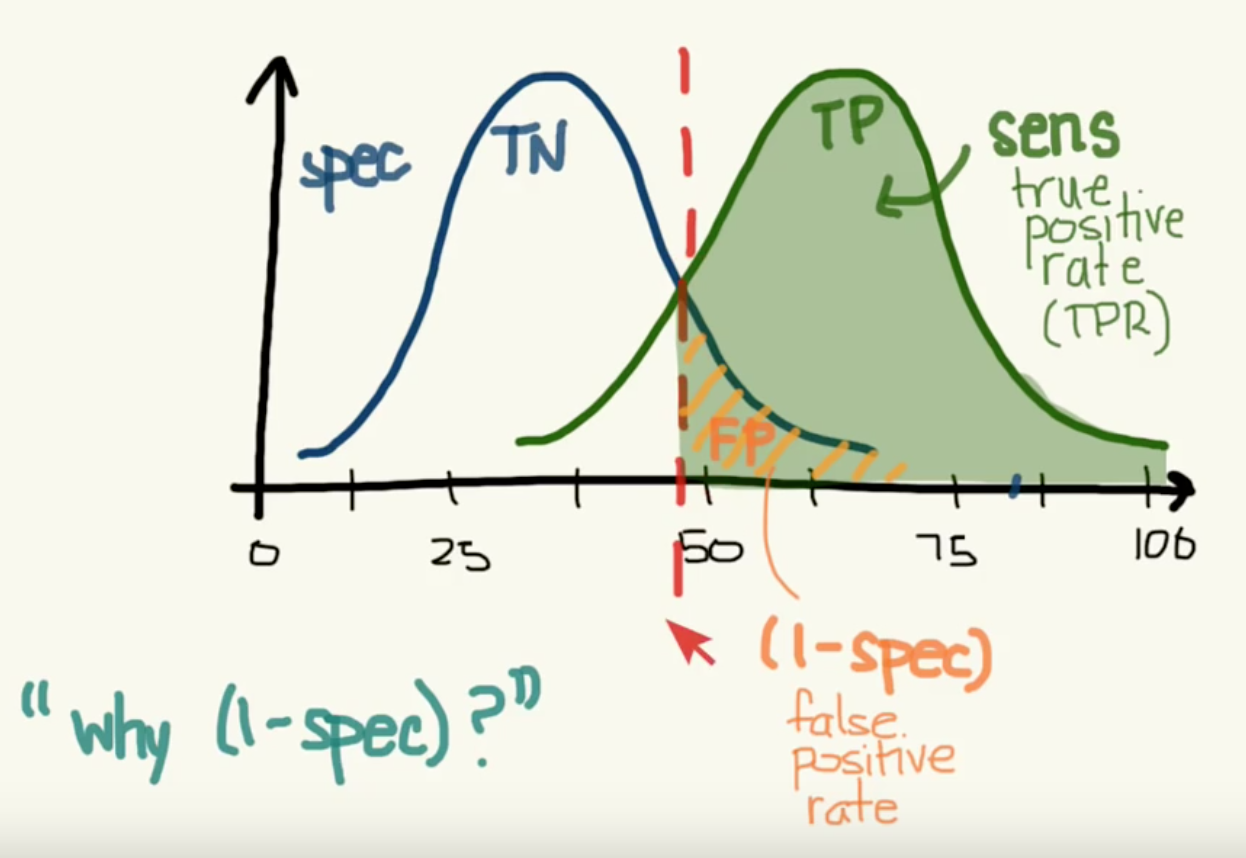
Recall|Sensitivity: (True Positive / [True Positive + False Negative]) High recall means to get all positives (i.e., True Positive + False Negative) despite having some false positives. Search & extraction in legal cases, Tumour detection. Often need humans to filter false positives.

Precision: (True Positive / [True Positive + False Positive]) High precision means it is important to filter off the any false positives. Search query suggestion, Document classification, customer-facing tasks.

F1-Score: is the harmonic mean of precision and sensitivity, ie., 2*((precision * recall) / (precision + recall))

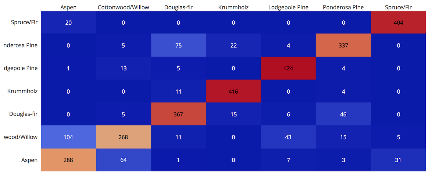
1. Confusion Matrix

Plain vanilla matrix. Not very useful as does not show the labels. However, the matrix can be used to build a heatmap using plotly directly.

print (sklearn.metrics.confusion_matrix(test_target,predictions))
array([[288,  64,   1,   0,   7,   3,  31],
       [104, 268,  11,   0,  43,  15,   5],
       [  0,   5, 367,  15,   6,  46,   0],
       [  0,   0,  11, 416,   0,   4,   0],
       [  1,  13,   5,   0, 424,   4,   0],
       [  0,   5,  75,  22,   4, 337,   0],
       [ 20,   0,   0,   0,   0,   0, 404]])

# make heatmap using plotly
from plotly.offline import iplot
from plotly.offline import init_notebook_mode
import plotly.graph_objs as go
init_notebook_mode(connected=True)

layout = go.Layout(width=800, height=400)
data = go.Heatmap(z=x,x=title,y=title)
fig = go.Figure(data=[data], layout=layout)
iplot(fig)

# this gives the values of each cell, but api unable to change the layout size
import plotly.figure_factory as ff
layout = go.Layout(width=800, height=500)
data = ff.create_annotated_heatmap(z=x,x=title,y=title)
iplot(data)

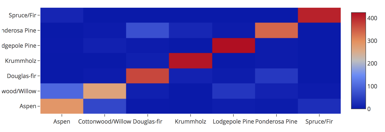
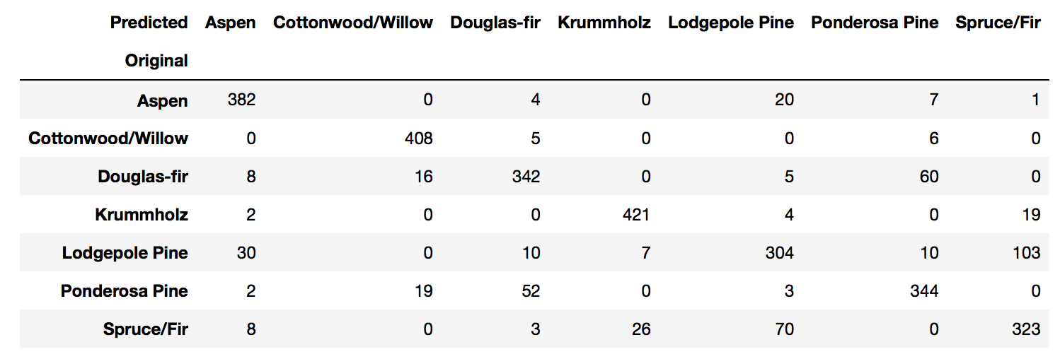
With pandas crosstab. Convert encoding into labels and put the two pandas series into a crosstab.

def forest(x):
  if x==1:
      return 'Spruce/Fir'
  elif x==2:
      return 'Lodgepole Pine'
  elif x==3:
      return 'Ponderosa Pine'
  elif x==4:
      return 'Cottonwood/Willow'
  elif x==5:
      return 'Aspen'
  elif x==6:
      return 'Douglas-fir'
  elif x==7:
      return 'Krummholz'

# Create pd Series for Original
# need to reset index as train_test is randomised
Original = test_target.apply(lambda x: forest(x)).reset_index(drop=True)
Original.name = 'Original'

# Create pd Series for Predicted
Predicted = pd.DataFrame(predictions, columns=['Predicted'])
Predicted = Predicted[Predicted.columns[0]].apply(lambda x: forest(x))

# Create Confusion Matrix
confusion = pd.crosstab(Original, Predicted)
confusion

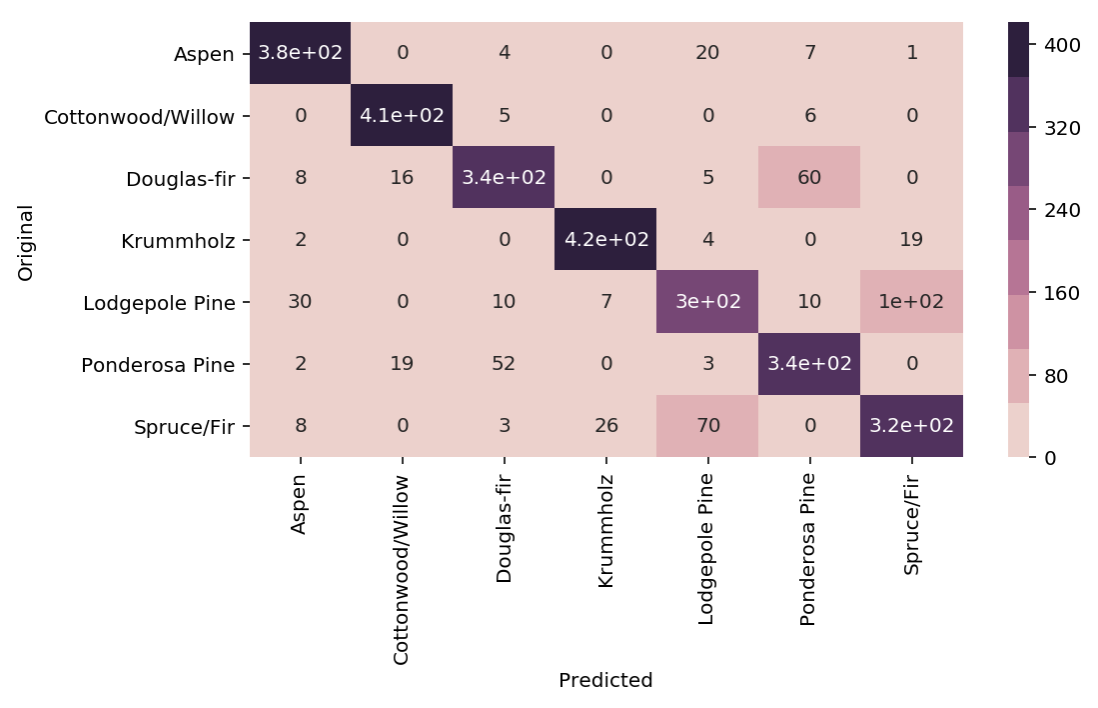
Using a heatmap.

# add confusion matrix from pd.crosstab earlier
plt.figure(figsize=(10, 5))
sns.heatmap(confusion,annot=True,cmap=sns.cubehelix_palette(8));

2. Evaluation Metrics

from sklearn.metrics import accuracy_score, precision_score, recall_score, f1_score

# Accuracy = TP + TN / (TP + TN + FP + FN)
# Precision = TP / (TP + FP)
# Recall = TP / (TP + FN)  Also known as sensitivity, or True Positive Rate
# F1 = 2 * (Precision * Recall) / (Precision + Recall)

print('Accuracy:', accuracy_score(y_test, tree_predicted)
print('Precision:', precision_score(y_test, tree_predicted)
print('Recall:', recall_score(y_test, tree_predicted)
print('F1:', f1_score(y_test, tree_predicted)

Accuracy: 0.95
Precision: 0.79
Recall: 0.60
F1: 0.68

# for precision/recall/f1 in multi-class classification
# need to add average=None or will prompt an error
# scoring will be for each label, and averaging them is necessary
from statistics import mean
mean(f1_score(y_test, y_predict, average=None))

There are many other evaluation metrics, a list can be found here:

from sklearn.metrics.scorer import SCORERS

for i in sorted(list(SCORERS.keys())):
    print i

accuracy
adjusted_rand_score
average_precision
f1
f1_macro
f1_micro
f1_samples
f1_weighted
log_loss
mean_absolute_error
mean_squared_error
median_absolute_error
neg_log_loss
neg_mean_absolute_error
neg_mean_squared_error
neg_median_absolute_error
precision
precision_macro
precision_micro
precision_samples
precision_weighted
r2
recall
recall_macro
recall_micro
recall_samples
recall_weighted
roc_auc

3. Classification Report

# Combined report with all above metrics
from sklearn.metrics import classification_report

print(classification_report(y_test, tree_predicted, target_names=['not 1', '1']))

              precision    recall  f1-score   support

      not 1       0.96      0.98      0.97       407
          1       0.79      0.60      0.68        43

avg / total       0.94      0.95      0.94       450

Classification report shows the details of precision, recall & f1-scores. It might be misleading to just print out a binary classification as their determination of True Positive, False Positive might differ from us. The report will tease out the details as shown below. We can also set average=None & compute the mean when printing out each individual scoring.

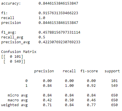
accuracy = accuracy_score(y_test, y_predict)
confusion = confusion_matrix(y_test,y_predict)
f1 = f1_score(y_test, y_predict)
recall = recall_score(y_test, y_predict)
precision = precision_score(y_test, y_predict)

f1_avg = mean(f1_score(y_test, y_predict, average=None))
recall_avg = mean(recall_score(y_test, y_predict, average=None))
precision_avg = mean(precision_score(y_test, y_predict, average=None))

print('accuracy:\t', accuracy)
print('\nf1:\t\t',f1)
print('recall\t\t',recall)
print('precision\t',precision)

print('\nf1_avg:\t\t',f1_avg)
print('recall_avg\t',recall_avg)
print('precision_avg\t',precision_avg)

print('\nConfusion Matrix')
print(confusion)
print('\n',classification_report(y_test, y_predict))

University of Michigan: Coursera Data Science in Python

4. Decision Function

X_train, X_test, y_train, y_test = train_test_split(X, y_binary_imbalanced, random_state=0)
y_scores_lr = lr.fit(X_train, y_train).decision_function(X_test)
y_score_list = list(zip(y_test[0:20], y_scores_lr[0:20]))

# show the decision_function scores for first 20 instances
y_score_list

[(0, -23.176682692580048),
 (0, -13.541079101203881),
 (0, -21.722576315155052),
 (0, -18.90752748077151),
 (0, -19.735941639551616),
 (0, -9.7494967330877031),
 (1, 5.2346395208185506),
 (0, -19.307366394398947),
 (0, -25.101037079396367),
 (0, -21.827003670866031),
 (0, -24.15099619980262),
 (0, -19.576751014363683),
 (0, -22.574837580426664),
 (0, -10.823683312193941),
 (0, -11.91254508661434),
 (0, -10.979579441354835),
 (1, 11.20593342976589),
 (0, -27.645821704614207),
 (0, -12.85921201890492),
 (0, -25.848618861971779)]

5. Probability Function

X_train, X_test, y_train, y_test = train_test_split(X, y_binary_imbalanced, random_state=0)
# note that the first column of array indicates probability of predicting negative class,
# 2nd column indicates probability of predicting positive class
y_proba_lr = lr.fit(X_train, y_train).predict_proba(X_test)
y_proba_list = list(zip(y_test[0:20], y_proba_lr[0:20,1]))

# show the probability of positive class for first 20 instances
y_proba_list

[(0, 8.5999236926158807e-11),
 (0, 1.31578065170999e-06),
 (0, 3.6813318939966053e-10),
 (0, 6.1456121155693793e-09),
 (0, 2.6840428788564424e-09),
 (0, 5.8320607398268079e-05),
 (1, 0.99469949997393026),
 (0, 4.1201906576825675e-09),
 (0, 1.2553305740618937e-11),
 (0, 3.3162918920398805e-10),
 (0, 3.2460530855408745e-11),
 (0, 3.1472051953481208e-09),
 (0, 1.5699022391384567e-10),
 (0, 1.9921654858205874e-05),
 (0, 6.7057057309326073e-06),
 (0, 1.704597440356912e-05),
 (1, 0.99998640688336282),
 (0, 9.8530840165646881e-13),
 (0, 2.6020404794341749e-06),
 (0, 5.9441185633886803e-12)]

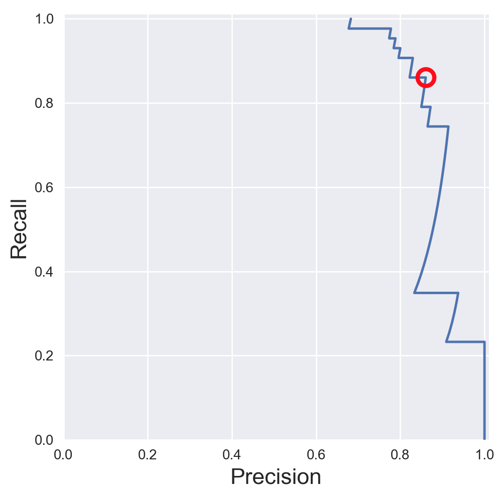
13.1.2. Precision-Recall Curves

If your problem involves kind of searching a needle in the haystack; the positive class samples are very rare compared to the negative classes, use a precision recall curve.

from sklearn.metrics import precision_recall_curve

# get decision function scores
y_scores_lr = m.fit(X_train, y_train).decision_function(X_test)

# get precision & recall values
precision, recall, thresholds = precision_recall_curve(y_test, y_scores_lr)
closest_zero = np.argmin(np.abs(thresholds))
closest_zero_p = precision[closest_zero]
closest_zero_r = recall[closest_zero]

plt.figure()
plt.xlim([0.0, 1.01])
plt.ylim([0.0, 1.01])
plt.plot(precision, recall, label='Precision-Recall Curve')
plt.plot(closest_zero_p, closest_zero_r, 'o', markersize = 12, fillstyle = 'none', c='r', mew=3)
plt.xlabel('Precision', fontsize=16)
plt.ylabel('Recall', fontsize=16)
plt.axes().set_aspect('equal')
plt.show()

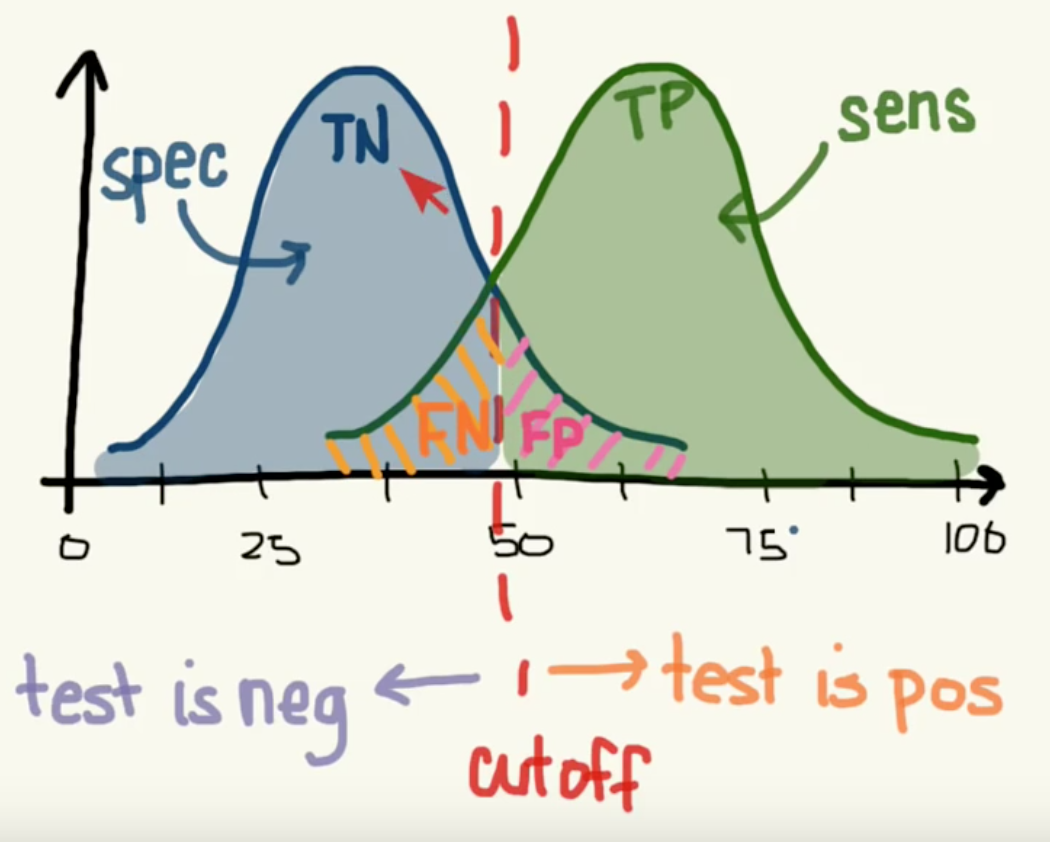
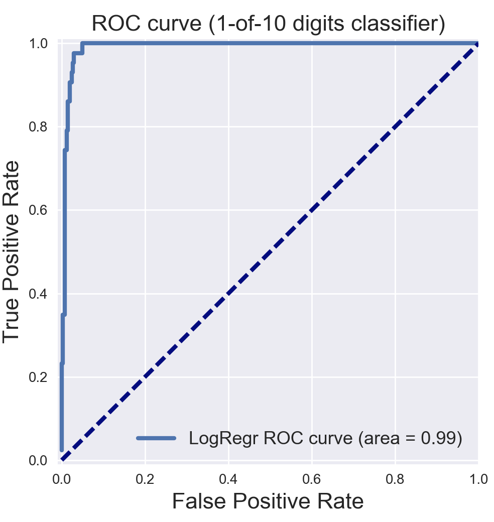
13.1.3. ROC Curves

Sensitivity vs 1-Specificity; or TP rate vs FP rate

Receiver Operating Characteristic (ROC) is used to show the performance of a binary classifier. Y-axis is True Positive Rate (Recall) & X-axis is False Positive Rate (Fall-Out). Area Under Curve (AUC) of a ROC is used. Higher AUC better.

The term came about in WWII where this metrics is used to determined a receiver operator’s ability to distinguish false positive and true postive correctly in the radar signals.

Some classifiers have a decision_function method while others have a probability prediction method, and some have both. Whichever one is available works fine for an ROC curve.

from sklearn.metrics import roc_curve, auc

X_train, X_test, y_train, y_test = train_test_split(X, y_binary_imbalanced, random_state=0)

y_score_lr = lr.fit(X_train, y_train).decision_function(X_test)
fpr_lr, tpr_lr, _ = roc_curve(y_test, y_score_lr)
roc_auc_lr = auc(fpr_lr, tpr_lr)

plt.figure()
plt.xlim([-0.01, 1.00])
plt.ylim([-0.01, 1.01])
plt.plot(fpr_lr, tpr_lr, lw=3, label='LogRegr ROC curve (area = {:0.2f})'.format(roc_auc_lr))
plt.xlabel('False Positive Rate', fontsize=16)
plt.ylabel('True Positive Rate', fontsize=16)
plt.title('ROC curve (1-of-10 digits classifier)', fontsize=16)
plt.legend(loc='lower right', fontsize=13)
plt.plot([0, 1], [0, 1], color='navy', lw=3, linestyle='--')
plt.axes().set_aspect('equal')
plt.show()

13.1.4. Log Loss

Logarithmic Loss, or Log Loss is a popular Kaggle evaluation metric, which measures the performance of a classification model where the prediction input is a probability value between 0 and 1

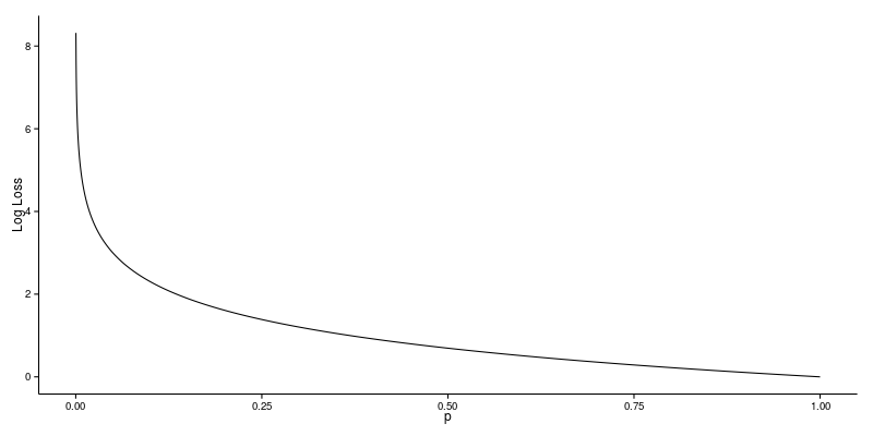
From datawookie

Log Loss quantifies the accuracy of a classifier by penalising false classifications; the catch is that Log Loss ramps up very rapidly as the predicted probability approaches 0. This article from datawookie gives a very good explanation.

13.2. Regression

For regression problems, where the response or y is a continuous value, it is common to use R-Squared and RMSE, or MAE as evaluation metrics. This website gives an excellent description on all the variants of errors metrics.

R-squared: Percentage of variability of dataset that can be explained by the model.

MSE. Mean squared error. Squaring then getting the mean of all errors (so change negatives into positives).

RMSE: Squared root of MSE so that it gives back the error at the same scale (as it was initially squared).

MAE: Mean Absolute Error. For negative errors, convert them to positive and obtain all error means.

The RMSE result will always be larger or equal to the MAE. If all of the errors have the same magnitude, then RMSE=MAE. Since the errors are squared before they are averaged, the RMSE gives a relatively high weight to large errors. This means the RMSE should be more useful when large errors are particularly undesirable.

from sklearn.metrics import mean_squared_error
from sklearn.metrics import mean_absolute_error

forest = RandomForestRegressor(n_estimators= 375)
model3 = forest.fit(X_train, y_train)
fullmodel = forest.fit(predictor, target)
print(model3)

# R2
r2_full = fullmodel.score(predictor, target)
r2_trains = model3.score(X_train, y_train)
r2_tests = model3.score(X_test, y_test)
print('\nr2 full:', r2_full)
print('r2 train:', r2_trains)
print('r2 test:', r2_tests)

# get predictions
y_predicted_total = model3.predict(predictor)
y_predicted_train = model3.predict(X_train)
y_predicted_test = model3.predict(X_test)

# get MSE
MSE_total = mean_squared_error(target, y_predicted_total)
MSE_train = mean_squared_error(y_train, y_predicted_train)
MSE_test = mean_squared_error(y_test, y_predicted_test)

# get RMSE by squared root
print('\nTotal RMSE:', np.sqrt(MSE_total))
print('Train RMSE:', np.sqrt(MSE_train))
print('Test RMSE:', np.sqrt(MSE_test))

# get MAE
MAE_total = mean_absolute_error(target, y_predicted_total)
MAE_train = mean_absolute_error(y_train, y_predicted_train)
MAE_test = mean_absolute_error(y_test, y_predicted_test)


# Train RMSE: 11.115272389673631
# Test RMSE: 34.872611746182706

# Train MAE 8.067078668023848
# Train MAE 24.541799999999995

RMSLE Root Mean Square Log Error is a very popular evaluation metric in data science competition now. It helps to reduce the effects of outliers compared to RMSE.

More: https://medium.com/analytics-vidhya/root-mean-square-log-error-rmse-vs-rmlse-935c6cc1802a

def rmsle(y, y0):
    assert len(y) == len(y0)
    return np.sqrt(np.mean(np.power(np.log1p(y)-np.log1p(y0), 2)))

13.3. K-fold Cross-Validation

Takes more time and computation to use k-fold, but well worth the cost. By default, sklearn uses stratified k-fold cross validation. Another type is ‘leave one out’ cross-validation.

The mean of the final scores among each k model is the most generalised output. This output can be compared to different model results for comparison.

More here.

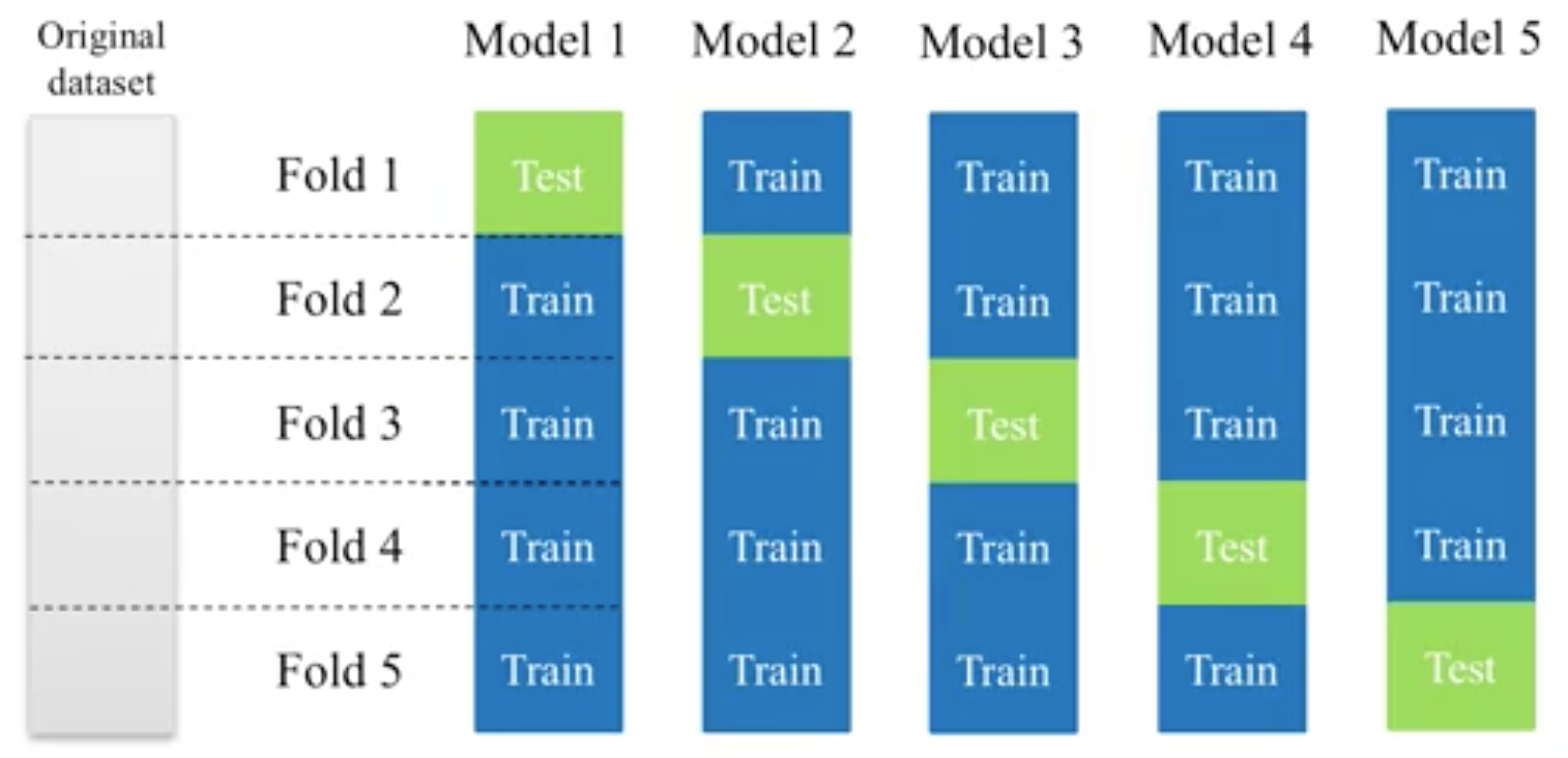
k-fold cross validation, with 5-folds

cross_val_score is a compact function to obtain the all scoring values using kfold in one line.

from sklearn.model_selection import cross_val_score
from sklearn.ensemble import RandomForestClassifier

X = df[df.columns[1:-1]]
y = df['Cover_Type']

# using 5-fold cross validation mean scores
model = RandomForestClassifier()
cv_scores = cross_val_score(model, X, y, scoring='accuracy', cv=5, n_jobs=-1)
print(np.mean(cv_scores))

For greater control, like to define our own evaluation metrics etc., we can use KFold to obtain the train & test indexes for each fold iteration.

from sklearn.model_selection import KFold
from sklearn.ensemble import RandomForestClassifier
from sklearn.metrics import f1_score

def kfold_custom(fold=4, X, y, model, eval_metric):
    kf = KFold(n_splits=4)
    score_total = []
    for train_index, test_index in kf.split(X):
        X_train, y_train = train[train_index][X_features], train[train_index][y_feature]
        X_test, y_test = test[test_index][X_features], test[test_index][y_feature]
        model.fit(X_train, y_train)
        y_predict = model.predict()
        score = eval_metric(y_test, y_predict)
        score_total.append(score)
    score = np.mean(score_total)
    return score

model = RandomForestClassifier()
kfold_custom(X, y, model, f1score)

There are many other variants of cross validations as shown below.

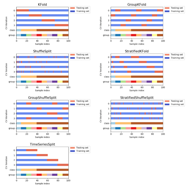
Types of cross-validation available in sklearn

13.4. Hyperparameters Tuning

There are generally 3 methods of hyperparameters tuning, i.e., Grid-Search, Random-Search, or the more automated Bayesian tuning.

13.4.1. Grid-Search

From Stackoverflow: Systematically working through multiple combinations of parameter tunes, cross validate each and determine which one gives the best performance. You can work through many combination only changing parameters a bit.

Print out the best_params_ and rebuild the model with these optimal parameters.

Simple example.

from sklearn.model_selection import GridSearchCV
from sklearn.ensemble import RandomForestClassifier

model = RandomForestClassifier()

grid_values = {'n_estimators':[150,175,200,225]}
grid = GridSearchCV(model, param_grid = grid_values, cv=5)
grid.fit(predictor, target)

print(grid.best_params_)
print(grid.best_score_)

# {'n_estimators': 200}
# 0.786044973545

Others.

from sklearn.svm import SVC
from sklearn.model_selection import GridSearchCV
from sklearn.metrics import roc_auc_score
from sklearn.model_selection import train_test_split


dataset = load_digits()
X, y = dataset.data, dataset.target == 1
X_train, X_test, y_train, y_test = train_test_split(X, y, random_state=0)

# choose a classifier
clf = SVC(kernel='rbf')

# input grid value range
grid_values = {'gamma': [0.001, 0.01, 0.05, 0.1, 1, 10, 100]}
# other parameters can be input in the dictionary, e.g.,
# grid_values = {'gamma': [0.01, 0.1, 1, 10], 'C': [0.01, 0.1, 1, 10]}
# OR n_estimators, max_features from RandomForest
# default metric to optimize over grid parameters: accuracy

grid_clf_acc = GridSearchCV(clf, param_grid = grid_values, random_state=0)

grid_clf_acc.fit(X_train, y_train)
y_decision_fn_scores_acc = grid_clf_acc.decision_function(X_test)

print('Grid best parameter (max. accuracy): ', grid_clf_acc.best_params_)
print('Grid best score (accuracy): ', grid_clf_acc.best_score_)

Using other scoring metrics

# alternative metric to optimize over grid parameters: AUC
# other scoring parameters include 'recall' or 'precision'
grid_clf_auc = GridSearchCV(clf, param_grid = grid_values, scoring = 'roc_auc', cv=3, random_state=0) # indicate AUC
grid_clf_auc.fit(X_train, y_train)
y_decision_fn_scores_auc = grid_clf_auc.decision_function(X_test)

print('Test set AUC: ', roc_auc_score(y_test, y_decision_fn_scores_auc))
print('Grid best parameter (max. AUC): ', grid_clf_auc.best_params_)
print('Grid best score (AUC): ', grid_clf_auc.best_score_)


# results 1
('Grid best parameter (max. accuracy): ', {'gamma': 0.001})
('Grid best score (accuracy): ', 0.99628804751299183)
# results 2
('Test set AUC: ', 0.99982858122393004)
('Grid best parameter (max. AUC): ', {'gamma': 0.001})
('Grid best score (AUC): ', 0.99987412783021423)


# gives break down of all permutations of gridsearch
print fittedmodel.cv_results_
# gives parameters that gives the best indicated scoring type
print CV.best_params_

13.4.2. Auto-Tuning

Bayesian Optimization as the name implies uses Bayesian optimization with Gaussian processes for autotuning. It is one of the most popular package now for auto-tuning. pip install bayesian-optimization

More: https://github.com/fmfn/BayesianOptimization

from bayes_opt import BayesianOptimization

# 1) Black box model function with output as evaluation metric

def cat_hyp(depth, learning_rate, bagging_temperature):
    params = {"iterations": 100,
              "eval_metric": "RMSE",
              "verbose": False,
              "depth": int(round(depth)),
              "learning_rate": learning_rate,
              "bagging_temperature": bagging_temperature}

    cat_feat = [] # Categorical features list
    cv_dataset = cgb.Pool(data=X, label=y, cat_features=cat_feat)

    # CV scores
    scores = catboost.cv(cv_dataset, params, fold_count=3)

    # negative as using RMSE, and optimizer tune to highest score
    return -np.max(scores['test-RMSE-mean'])


# 2) Bounded region of parameter space
pbounds = {'depth': (2, 10),
           'bagging_temperature': (3,10),
           'learning_rate': (0.05,0.9)}

# 3) Define optimizer function
optimizer = BayesianOptimization(f=black_box_function,
                                 pbounds=pbounds,
                                 random_state=1)

# 4) Start optimizing
    # init_points: no. steps of random exploration. Helps to diversify random space
    # n_iter: no. steps for bayesian optimization. Helps to exploit learnt parameters
optimizer.maximize(init_points=2, n_iter=3)

# 5) Get best parameters
best_param = optimizer.max['params']

Here’s another example using Random Forest

from bayes_opt import BayesianOptimization
from sklearn.ensemble import RandomForestRegressor

def rmsle(y, y0):
    assert len(y) == len(y0)
    return np.sqrt(np.mean(np.power(np.log1p(y)-np.log1p(y0), 2)))

def black_box(n_estimators, max_depth):
    params = {"n_jobs": 5,
              "n_estimators": int(round(n_estimators)),
              "max_depth": max_depth}

    model = RandomForestRegressor(**params)
    model.fit(X_train, y_train)
    y_predict = model.predict(X_test)
    score = rmsle(y_test, y_predict)

    return -score

# Search space
pbounds = {'n_estimators': (1, 5),
           'max_depth': (10,50)}

optimizer = BayesianOptimization(black_box, pbounds, random_state=2100)
optimizer.maximize(init_points=10, n_iter=5)
best_param = optimizer.max['params']

Bayesian Tuning and Bandits (BTB) is a package used for auto-tuning ML models hyperparameters. It similarly uses Gaussian Process to do this, though there is an option for Uniform. It was born from a Master thesis by Laura Gustafson in 2018. Because it is lower level than the above package, it has better flexibility, e.g., defining a k-fold cross-validation.

https://github.com/HDI-Project/BTB

from btb.tuning import GP
from btb import HyperParameter, ParamTypes

# remember to change INT to FLOAT where necessary
tunables = [('n_estimators', HyperParameter(ParamTypes.INT, [500, 2000])),
            ('max_depth', HyperParameter(ParamTypes.INT, [3, 20]))]

def auto_tuning(tunables, epoch, X_train, X_test, y_train, y_test, verbose=0):
    """Auto-tuner using BTB library"""
    tuner = GP(tunables)
    parameters = tuner.propose()

    score_list = []
    param_list = []

    for i in range(epoch):
        # ** unpacks dict in a argument
        model = RandomForestClassifier(**parameters, n_jobs=-1)
        model.fit(X_train, y_train)
        y_predict = model.predict(X_test)
        score = accuracy_score(y_test, y_predict)

        # store scores & parameters
        score_list.append(score)
        param_list.append(parameters)

        if verbose==0:
            pass
        elif verbose==1:
            print('epoch: {}, accuracy: {}'.format(i+1,score))
        elif verbose==2:
            print('epoch: {}, accuracy: {}, param: {}'.format(i+1,score,parameters))

        # get new parameters
        tuner.add(parameters, score)
        parameters = tuner.propose()

    best_s = tuner._best_score
    best_score_index = score_list.index(best_s)
    best_param = param_list[best_score_index]
    print('\nbest accuracy: {}'.format(best_s))
    print('best parameters: {}'.format(best_param))
    return best_param

best_param = auto_tuning(tunables, 5, X_train, X_test, y_train, y_test)

# epoch: 1, accuracy: 0.7437106918238994
# epoch: 2, accuracy: 0.779874213836478
# epoch: 3, accuracy: 0.7940251572327044
# epoch: 4, accuracy: 0.7908805031446541
# epoch: 5, accuracy: 0.7987421383647799

# best accuracy: 0.7987421383647799
# best parameters: {'n_estimators': 1939, 'max_depth': 18}

For regression models, we have to make some slight modifications, since the optimization of hyperparameters is tuned towards a higher evaluation score.

from btb.tuning import GP
from btb import HyperParameter, ParamTypes
from sklearn.metrics import mean_squared_error

def auto_tuning(tunables, epoch, X_train, X_test, y_train, y_test, verbose=1):
    """Auto-tuner using BTB library"""
    tuner = GP(tunables)
    parameters = tuner.propose()

    score_list = []
    param_list = []

    for i in range(epoch):
        model = RandomForestRegressor(**parameters, n_jobs=10, verbose=3)
        model.fit(X_train, y_train)
        y_predict = model.predict(X_test)
        score = np.sqrt(mean_squared_error(y_test, y_predict))

        # store scores & parameters
        score_list.append(score)
        param_list.append(parameters)

        if verbose==0:
            pass
        elif verbose==1:
            print('epoch: {}, rmse: {}, param: {}'.format(i+1,score,parameters))

        # BTB tunes parameters based the logic on higher score = good
        # but RMSE is lower the better, hence need to change scores to negative to inverse it
        score = -score

        # get new parameters
        tuner.add(parameters, score)
        parameters = tuner.propose()

    best_s = tuner._best_score
    best_score_index = score_list.index(best_s)
    best_param = param_list[best_score_index]
    print('\nbest rmse: {}'.format(best_s))
    print('best parameters: {}'.format(best_param))
    return best_param

Auto-Sklearn is another auto-ml package that automatically selects both the model and its hyperparameters.

https://automl.github.io/auto-sklearn/master/

import autosklearn.classification
import sklearn.model_selection
import sklearn.datasets
import sklearn.metrics

X, y = sklearn.datasets.load_digits(return_X_y=True)
X_train, X_test, y_train, y_test = sklearn.model_selection.train_test_split(X, y, random_state=1)

automl = autosklearn.classification.AutoSklearnClassifier()
automl.fit(X_train, y_train)

y_pred = automl.predict(X_test)
print("Accuracy score", sklearn.metrics.accuracy_score(y_test, y_pred))

Auto Keras uses neural network for training. Similar to Google’s AutoML approach.

import autokeras as ak

clf = ak.ImageClassifier()
clf.fit(x_train, y_train)
results = clf.predict(x_test)