11. Deep Learning
Deep Learning falls under the broad class of Articial Intelligence > Machine Learning. It is a Machine Learning technique that uses multiple internal layers (hidden layers) of non-linear processing units (neurons) to conduct supervised or unsupervised learning from data.
11.1. Introduction
11.1.1. GPU
Tensorflow is able to run faster and more effeciently using Nivida’s GPU pip install tensorflow-gpu.
CUDA as well cudnn are also required. It is best to run your models in Ubuntu as the compliation of
some pretrained models are easier.
11.1.2. Preprocessing
Keras accepts numpy input, so we have to convert. Also, for multi-class classification,
we need to convert them into binary values; i.e., using one-hot encoding. For the latter, we can in-place use
sparse_categorical_crossentropy for the loss function which will can
process the multi-class label without converting to one-hot encoding.
# convert to numpy arrays
X = np.array(X)
# OR
X = X.values

# one-hot encoding for multi-class y labels
Y = pd.get_dummies(y)
It is important to scale or normalise the dataset before putting in the neural network.
from sklearn.preprocessing import StandardScaler

X_train, X_test, y_train, y_test = train_test_split(X, y,
                                                    random_state = 0)
scaler = StandardScaler()
X_train = scaler.fit_transform(X_train)
X_test = scaler.transform(X_test)
Model architecture can also be displayed in a graph. Or we can print as a summary
from IPython.display import SVG
from tensorflow.python.keras.utils.vis_utils import model_to_dot

SVG(model_to_dot(model, show_shapes=True).create(prog='dot', format='svg'))
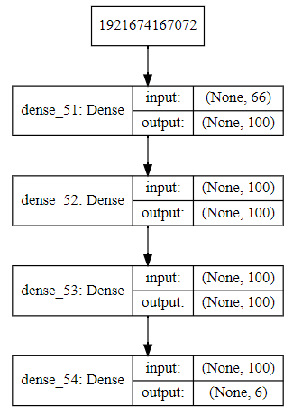
model architecture printout
model.summary()
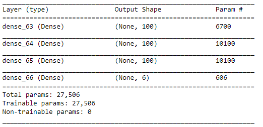
model summary printout
11.1.3. Evaluation
The model compiled has a history method (model.history.history) that gives the accuracy and loss for both train & test sets for each time step.
We can plot it out for a better visualization. Alternatively we can also use TensorBoard, which is installed together with TensorFlow package.
It will also draw the model architecture.
def plot_validate(model, loss_acc):
    '''Plot model accuracy or loss for both train and test validation per epoch
    model = fitted model
    loss_acc = input 'loss' or 'acc' to plot respective graph
    '''
    history = model.history.history

    if loss_acc == 'loss':
        axis_title = 'loss'
        title = 'Loss'
        epoch = len(history['loss'])
    elif loss_acc == 'acc':
        axis_title = 'acc'
        title = 'Accuracy'
        epoch = len(history['loss'])

    plt.figure(figsize=(15,4))
    plt.plot(history[axis_title])
    plt.plot(history['val_' + axis_title])
    plt.title('Model ' + title)
    plt.ylabel(title)
    plt.xlabel('Epoch')

    plt.grid(b=True, which='major')
    plt.minorticks_on()
    plt.grid(b=True, which='minor', alpha=0.2)

    plt.legend(['Train', 'Test'])
    plt.show()


plot_validate(model, 'acc')
plot_validate(model, 'loss')

11.1.4. Auto-Tuning
Unlike grid-search we can use Bayesian optimization for a faster hyperparameter tuning.
https://www.dlology.com/blog/how-to-do-hyperparameter-search-with-baysian-optimization-for-keras-model/ https://medium.com/@crawftv/parameter-hyperparameter-tuning-with-bayesian-optimization-7acf42d348e1
11.2. Model Compiling
11.2.1. Activation Functions
11.2.1.2. Output Layer
Activation function
- Binary Classification: Sigmoid
- Multi-Class Classification: Softmax
- Regression: Linear
11.2.2. Gradient Descent
Backpropagation, short for “backward propagation of errors,” is an algorithm for supervised learning of artificial neural networks using gradient descent.
- Optimizer is a learning algorithm called gradient descent, refers to the calculation of an error gradient or slope of error and “descent” refers to the moving down along that slope towards some minimum level of error.
- Batch Size is a hyperparameter of gradient descent that controls the number of training samples to work through before the model’s internal parameters are updated.
- Epoch is a hyperparameter of gradient descent that controls the number of complete passes through the training dataset.
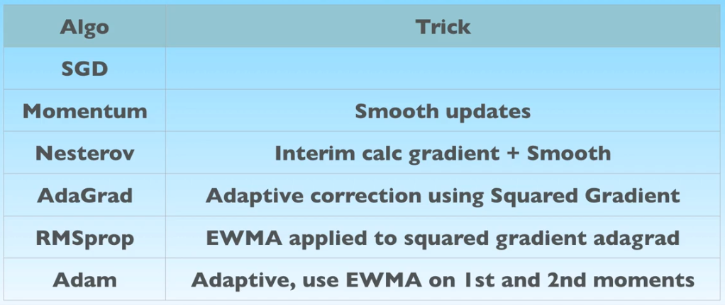
Optimizers is used to find the minimium value of the cost function to perform backward propagation. There are more advanced adaptive optimizers, like AdaGrad/RMSprop/Adam, that allow the learning rate to adapt to the size of the gradient. The hyperparameters are essential to get the model to perform well.
The amount that the weights are updated during training is referred to as the step size or the “learning rate.” Specifically, the learning rate is a configurable hyperparameter used in the training of neural networks that has a small positive value, often in the range between 0.0 and 1.0. A learning rate that is too large can cause the model to converge too quickly to a suboptimal solution, whereas a learning rate that is too small can cause the process to get stuck. (https://machinelearningmastery.com/understand-the-dynamics-of-learning-rate-on-deep-learning-neural-networks/)
From Udemy, Zero to Hero Deep Learning with Python & Keras
Assume you have a dataset with 200 samples (rows of data) and you choose a batch size of 5 and 1,000 epochs. This means that the dataset will be divided into 40 batches, each with 5 samples. The model weights will be updated after each batch of 5 samples. This also means that one epoch will involve 40 batches or 40 updates to the model.
11.3. ANN
11.3.1. Theory
An artifical neural network is the most basic form of neural network. It consists of an input layer, hidden layers, and an output layer. This writeup by Berkeley gave an excellent introduction to the theory. Most of the diagrams are taken from the site.
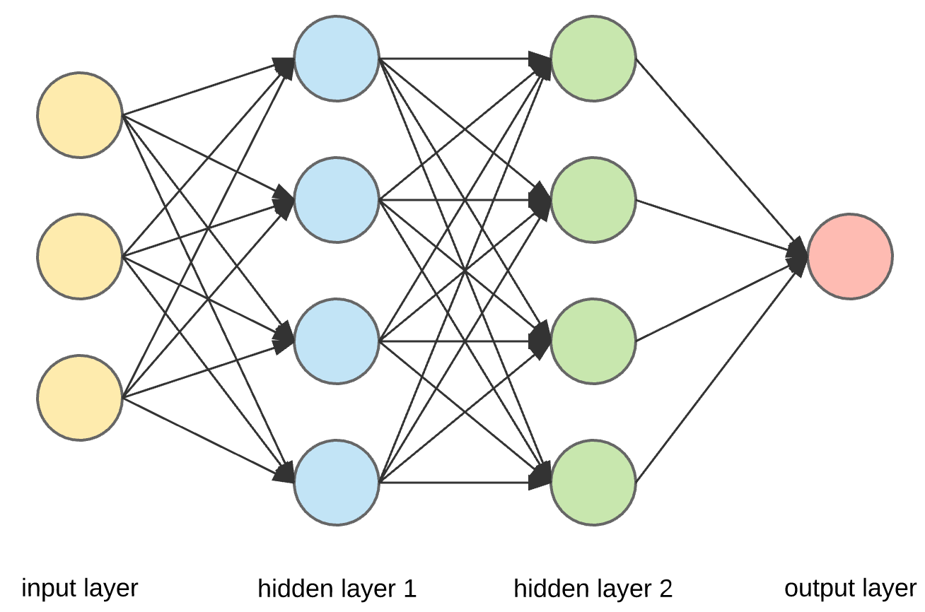
Structure of an artificial neutral network
Zooming in at a single perceptron, the input layer consists of every individual features, each with an assigned weight feeding to the hidden layer. An activation function tells the perception what outcome it is.
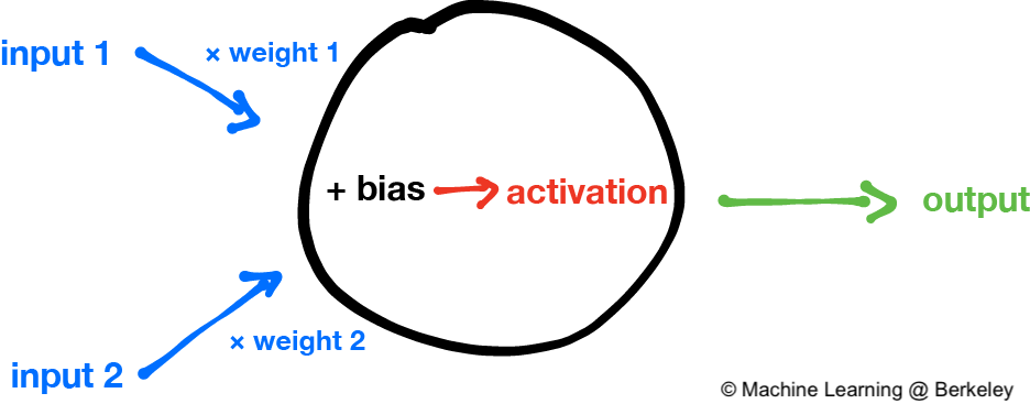
Structure of a single perceptron
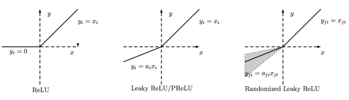
Activation functions consists of ReLU, Tanh, Linear, Sigmoid, Softmax and many others. Sigmoid is used for binary classifications, while softmax is used for multi-class classifications.
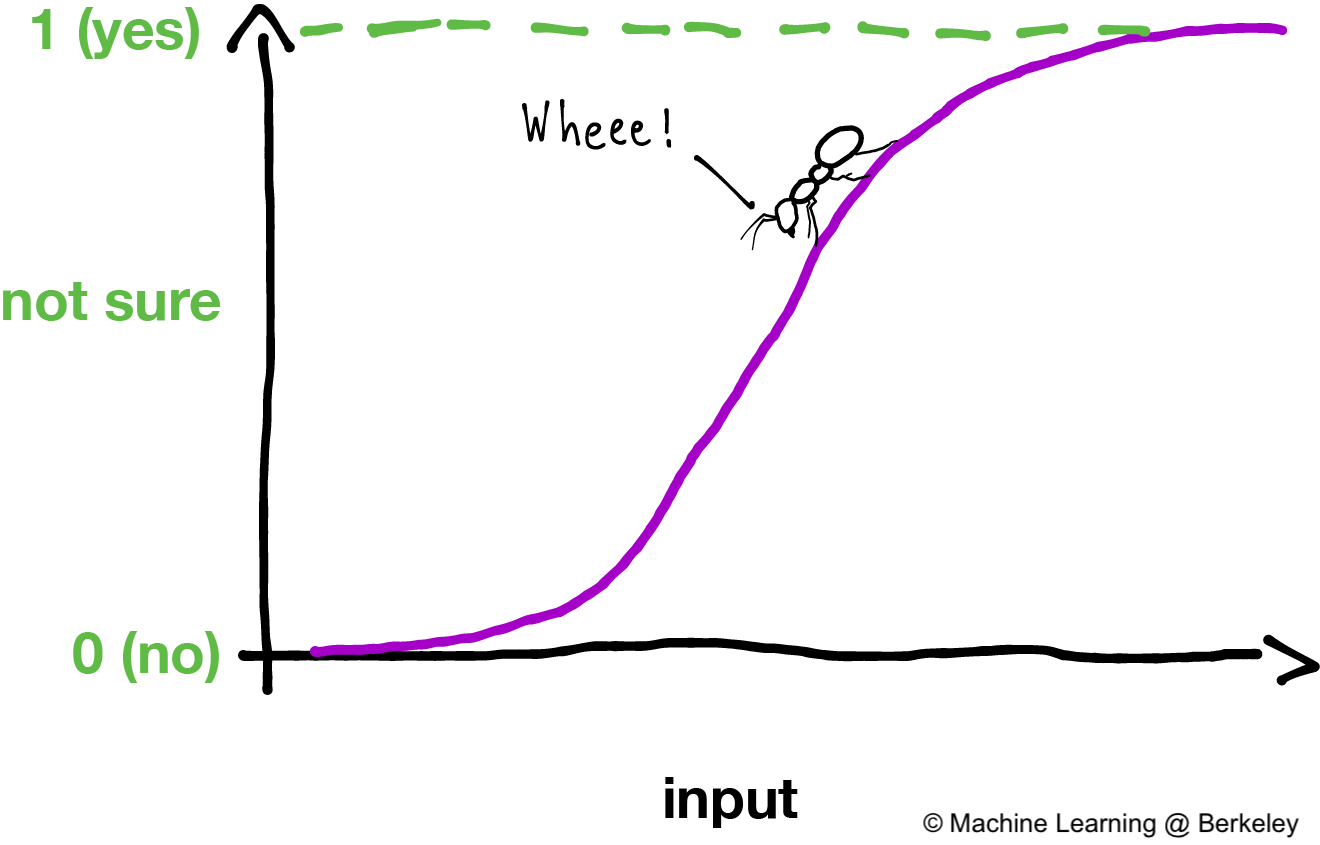
An activation function, using sigmoid function
The backward propagation algorithm works in such that the slopes of gradient descent is calculated by working backwards from the output layer back to the input layer. The weights are readjusted to reduce the loss and improve the accuracy of the model.
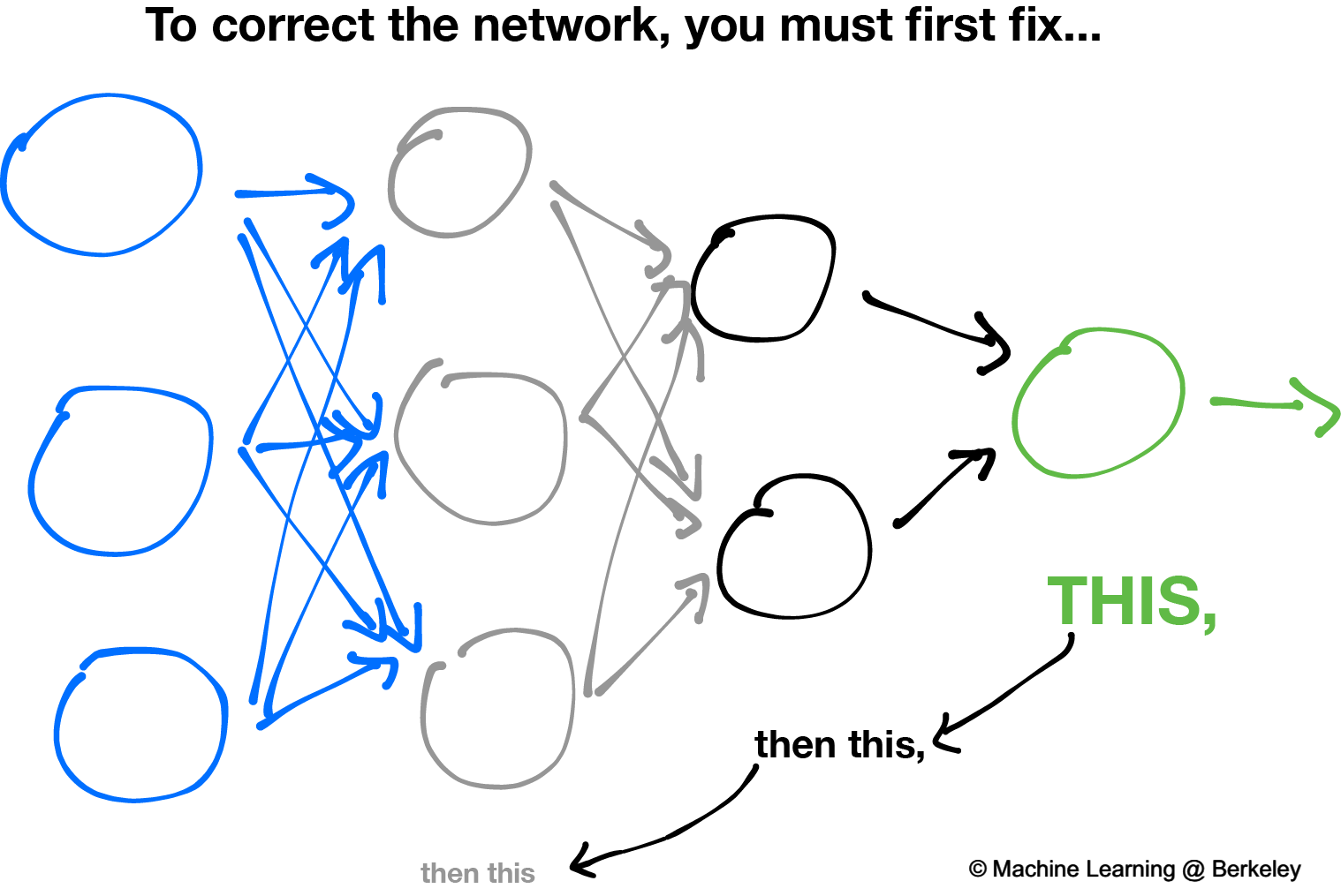
Backward propagation
A summary is as follows
- Randomly initialize the weights for all the nodes.
- For every training example, perform a forward pass using the current weights, and calculate the output of each node going from left to right. The final output is the value of the last node.
- Compare the final output with the actual target in the training data, and measure the error using a loss function.
- Perform a backwards pass from right to left and propagate the error to every individual node using backpropagation. Calculate each weight’s contribution to the error, and adjust the weights accordingly using gradient descent. Propagate the error gradients back starting from the last layer.
11.3.2. Keras Model
- Building an ANN model in Keras library requires
- input & hidden layers
- model compliation
- model fitting
- model evalution
Definition of layers are typically done using the typical Dense layer, or regularization layer called Dropout. The latter prevents overfitting as it randomly selects neurons to be ignored during training.
from tensorflow.keras.models import Sequential
from tensorflow.keras.layers import Dense, Dropout

# using dropout layers
model = Sequential()
model.add(Dense(512, activation='relu', input_shape=(784,)))
model.add(Dropout(0.2))
model.add(Dense(512, activation='relu'))
model.add(Dropout(0.2))
model.add(Dense(10, activation='softmax'))
Before training, the model needs to be compiled with the learning hyperparameters of optimizer, loss, and metric functions.
# from keras documentation
# https://keras.io/getting-started/sequential-model-guide/

# For a multi-class classification problem
model.compile(optimizer='rmsprop',
              loss='categorical_crossentropy',
              metrics=['accuracy'])

# For a binary classification problem
model.compile(optimizer='rmsprop',
              loss='binary_crossentropy',
              metrics=['accuracy'])

# For a mean squared error regression problem
model.compile(optimizer='rmsprop',
              loss='mse')


# we can also set optimizer's parameters
from tensorflow.keras.optimizers import RMSprop
rmsprop = RMSprop(lr=0.001, rho=0.9, epsilon=None, decay=0.0)
model.compile(optimizer=rmsprop, loss='mse')
We can also use sklearn’s cross-validation.
from tensorflow.keras.layers import Dense
from tensorflow.keras.models import Sequential

def create_model():
    model = Sequential()
    model.add(Dense(6, input_dim=4, kernel_initializer='normal', activation='relu'))
    #model.add(Dense(4, kernel_initializer='normal', activation='relu'))
    model.add(Dense(1, kernel_initializer='normal', activation='sigmoid'))
    model.compile(loss='binary_crossentropy', optimizer='adam', metrics=['accuracy'])
    return model

from sklearn.model_selection import cross_val_score
from tensorflow.keras.wrappers.scikit_learn import KerasClassifier

# Wrap our Keras model in an estimator compatible with scikit_learn
estimator = KerasClassifier(build_fn=create_model, epochs=100, verbose=0)
cv_scores = cross_val_score(estimator, all_features_scaled, all_classes, cv=10)
cv_scores.mean()
The below gives a compiled code example code.
from tensorflow import keras
from tensorflow.keras.datasets import mnist
from tensorflow.keras.models import Sequential
from tensorflow.keras.layers import Dense, Dropout
from tensorflow.keras.optimizers import RMSprop

(mnist_train_images, mnist_train_labels), (mnist_test_images, mnist_test_labels) = mnist.load_data()

train_images = mnist_train_images.reshape(60000, 784)
test_images = mnist_test_images.reshape(10000, 784)
train_images = train_images.astype('float32')
test_images = test_images.astype('float32')
train_images /= 255
test_images /= 255

# convert the 0-9 labels into "one-hot" format, as we did for TensorFlow.
train_labels = keras.utils.to_categorical(mnist_train_labels, 10)
test_labels = keras.utils.to_categorical(mnist_test_labels, 10)


model = Sequential()
model.add(Dense(512, activation='relu', input_shape=(784,)))
model.add(Dense(10, activation='softmax'))
model.summary()


Layer (type)                 Output Shape              Param #
=================================================================
dense (Dense)                (None, 512)               401920
_________________________________________________________________
dense_1 (Dense)              (None, 10)                5130
=================================================================
Total params: 407,050
Trainable params: 407,050
Non-trainable params: 0
_________________________________________________________________

model.compile(loss='categorical_crossentropy',
                optimizer=RMSprop(),
                metrics=['accuracy'])


history = model.fit(train_images, train_labels,
                    batch_size=100, #no of samples per gradient update
                    epochs=10, #iteration
                    verbose=1, #0=no printout, 1=progress bar, 2=step-by-step printout
                    validation_data=(test_images, test_labels))

# Train on 60000 samples, validate on 10000 samples
# Epoch 1/10
# - 4s - loss: 0.2459 - acc: 0.9276 - val_loss: 0.1298 - val_acc: 0.9606
# Epoch 2/10
# - 4s - loss: 0.0991 - acc: 0.9700 - val_loss: 0.0838 - val_acc: 0.9733
# Epoch 3/10
# - 4s - loss: 0.0656 - acc: 0.9804 - val_loss: 0.0738 - val_acc: 0.9784
# Epoch 4/10
# - 4s - loss: 0.0493 - acc: 0.9850 - val_loss: 0.0650 - val_acc: 0.9798
# Epoch 5/10
# - 4s - loss: 0.0367 - acc: 0.9890 - val_loss: 0.0617 - val_acc: 0.9817
# Epoch 6/10
# - 4s - loss: 0.0281 - acc: 0.9915 - val_loss: 0.0698 - val_acc: 0.9800
# Epoch 7/10
# - 4s - loss: 0.0221 - acc: 0.9936 - val_loss: 0.0665 - val_acc: 0.9814
# Epoch 8/10
# - 4s - loss: 0.0172 - acc: 0.9954 - val_loss: 0.0663 - val_acc: 0.9823
# Epoch 9/10
# - 4s - loss: 0.0128 - acc: 0.9964 - val_loss: 0.0747 - val_acc: 0.9825
# Epoch 10/10
# - 4s - loss: 0.0098 - acc: 0.9972 - val_loss: 0.0840 - val_acc: 0.9795


score = model.evaluate(test_images, test_labels, verbose=0)
print('Test loss:', score[0])
print('Test accuracy:', score[1])
Here’s another example using the Iris dataset.
import pandas as pd
import numpy as np

from keras.models import Sequential
from keras.layers import Dense, Dropout, Activation
from sklearn.model_selection import train_test_split
from sklearn.datasets import load_iris
import matplotlib.pyplot as plt


def modeling(X_train, y_train, X_test, y_test, features, classes, epoch, batch, verbose, dropout):

    model = Sequential()

    #first layer input dim as number of features
    model.add(Dense(100, activation='relu', input_dim=features))
    model.add(Dropout(dropout))
    model.add(Dense(50, activation='relu'))
    #nodes must be same as no. of labels classes
    model.add(Dense(classes, activation='softmax'))

    model.compile(loss='sparse_categorical_crossentropy',
                    optimizer='adam',
                    metrics=['accuracy'])

    model.fit(X_train, y_train,
            batch_size=batch,
            epochs= epoch,
            verbose=verbose,
            validation_data=(X_test, y_test))

    return model

iris = load_iris()
X = pd.DataFrame(iris['data'], columns=iris['feature_names'])
y = iris.target
X_train, X_test, y_train, y_test = train_test_split(X,y,random_state=0)

# define ANN model parameters
features = X_train.shape[1]
classes = len(np.unique(y_train))
epoch = 100
batch = 25
verbose = 0
dropout = 0.2

model = modeling(X_train, y_train, X_test, y_test, features, classes, epoch, batch, verbose, dropout)
11.4. CNN
Convolutional Neural Network (CNN) is suitable for unstructured data like image classification, machine translation, sentence classification, and sentiment analysis.
11.4.1. Theory
This article from medium gives a good introduction of CNN. The steps goes something like this:
- Provide input image into convolution layer
- Choose parameters, apply filters with strides, padding if requires. Perform convolution on the image and apply ReLU activation to the matrix.
- Perform pooling to reduce dimensionality size. Max-pooling is most commonly used
- Add as many convolutional layers until satisfied
- Flatten the output and feed into a fully connected layer (FC Layer)
- Output the class using an activation function (Logistic Regression with cost functions) and classifies images.
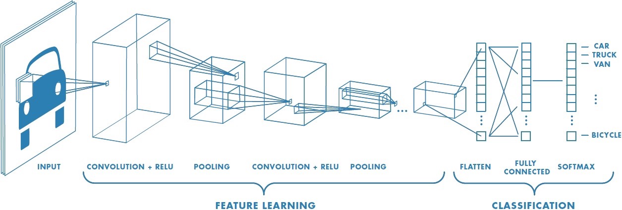
from medium
There are many topologies, or CNN architecture to build on as the hyperparameters, layers etc. are endless. Some specialized architecture includes LeNet-5 (handwriting recognition), AlexNet (deeper than LeNet, image classification), GoogLeNet (deeper than AlexNet, includes inception modules, or groups of convolution), ResNet (even deeper, maintains performance using skip connections). This article1 gives a good summary of each architecture.
11.4.2. Keras Model
import tensorflow
from tensorflow.keras.datasets import mnist
from tensorflow.keras.models import Sequential
from tensorflow.keras.layers import Dense, Dropout, Conv2D, MaxPooling2D, Flatten
from tensorflow.keras.optimizers import RMSprop

(X_train, y_train), (X_test, y_test) = mnist.load_data()


# need to reshape image dataset
total_rows_train = X_train.shape[0]
total_rows_test = X_test.shape[0]
sample_rows = X_train.shape[1]
sample_columns = X_train.shape[2]
num_channels = 1

# i.e. X_train = X_train.reshape(60000,28,28,1), where 1 means images are grayscale
X_train = X_train.reshape(total_rows_train, sample_rows, sample_columns, num_channels)
X_test = X_test.reshape(total_rows_test, sample_rows, sample_columns, num_channels)


model = Sequential()
model.add(Conv2D(32, kernel_size=(3, 3), activation='relu',
                 input_shape=(sample_rows, sample_columns, num_channels)))

# 64 3x3 kernels
model.add(Conv2D(64, (3, 3), activation='relu'))
# Reduce by taking the max of each 2x2 block
model.add(MaxPooling2D(pool_size=(2, 2)))
# Dropout to avoid overfitting
model.add(Dropout(0.25))
# Flatten the results to one dimension for passing into our final layer
model.add(Flatten())
# A hidden layer to learn with
model.add(Dense(128, activation='relu'))
# Another dropout
model.add(Dropout(0.5))
# Final categorization from 0-9 with softmax
model.add(Dense(10, activation='softmax'))


model.summary()

# _________________________________________________________________
# Layer (type)                 Output Shape              Param #
# =================================================================
# conv2d (Conv2D)              (None, 26, 26, 32)        320
# _________________________________________________________________
# conv2d_1 (Conv2D)            (None, 24, 24, 64)        18496
# _________________________________________________________________
# max_pooling2d (MaxPooling2D) (None, 12, 12, 64)        0
# _________________________________________________________________
# dropout (Dropout)            (None, 12, 12, 64)        0
# _________________________________________________________________
# flatten (Flatten)            (None, 9216)              0
# _________________________________________________________________
# dense (Dense)                (None, 128)               1179776
# _________________________________________________________________
# dropout_1 (Dropout)          (None, 128)               0
# _________________________________________________________________
# dense_1 (Dense)              (None, 10)                1290
# =================================================================
# Total params: 1,199,882
# Trainable params: 1,199,882
# Non-trainable params: 0
# _________________________________________________________________

model.compile(loss='sparse_categorical_crossentropy',
          optimizer='adam',
          metrics=['accuracy'])

history = model.fit(train_images, train_labels,
                    batch_size=32,
                    epochs=10,
                    verbose=1,
                    validation_data=(test_images, test_labels))

score = model.evaluate(test_images, test_labels, verbose=0)
print('Test loss:', score[0])
print('Test accuracy:', score[1])

# Test loss: 0.034049834153382426
# Test accuracy: 0.9918
11.4.3. Image Augmentation
It is hard to obtain photogenic samples of every aspect. Image augmentation enables the auto-generation of new samples from existing ones through random adjustment from rotation, shifts, zoom, brightness etc. The below samples pertains to increasing samples when all samples in classes are balanced.
from keras_preprocessing.image import ImageDataGenerator

train_aug = ImageDataGenerator(rotation_range=360, # Degree range for random rotations
                                width_shift_range=0.2, # Range for random horizontal shifts
                                height_shift_range=0.2, # Range for random vertical shifts
                                zoom_range=0.2, # Range for random zoom
                                horizontal_flip=True, # Randomly flip inputs horizontally
                                vertical_flip=True, # Randomly flip inputs vertically
                                brightness_range=[0.5, 1.5])

# we should not augment validation and testing samples
val_aug = ImageDataGenerator()
test_aug = ImageDataGenerator()
After setting the augmentation settings, we will need to decide how to “flow” the data, original samples
into the model. In this function, we can also resize the images automatically if necessary.
Finally to fit the model, we use the model.fit_generator function so that for every epoch,
the full original samples will be augmented randomly on the fly.
They will not be stored in memory for obvious reasons.
Essentially, there are 3 ways to do this.
First, we can flow the images from memory flow, which means we have to load the data in memory first.
batch_size = 32
img_size = 100

train_flow = train_aug.flow(X_train, Y_train,
                            target_size=(img_size,img_size),
                            batch_size=batch_size)

val_flow = val_aug.flow(X_val, Y_val,
                        target_size=(img_size,img_size),
                        batch_size=batch_size)

model.fit_generator(train_flow,
                    steps_per_epoch=32,
                    epochs=15,
                    verbose=1,
                    validation_data=val_flow,
                    use_multiprocessing=True,
                    workers=2)
Second, we can flow the images from a directory flow_from_dataframe,
where all classes of images are in that single directory.
This requires a dataframe which indicates which image correspond to which class.
dir = r'/kaggle/input/plant-pathology-2020-fgvc7/images'
train_flow = train_aug.flow_from_dataframe(train_df,
                                            directory=dir,
                                            x_col='image_name',
                                            y_col=['class1','class2','class3','class4'],
                                            class_mode='categorical'
                                            batch_size=batch_size)
Third, we can flow the images from a main directory flow_from_directory,
where all each class of images are in individual subdirectories.
# to include all subdirectories' images, no need specific classes
train_flow = train_aug.flow_from_directory(directory=dir,
                                            class_mode='categorical',
                                            target_size=(img_size,img_size),
                                            batch_size=32)

# to include specific subdirectories' images, put list of subdirectory names under classes
train_flow = train_aug.flow_from_directory(directory=dir,
                                            classes=['subdir1', 'subdir2', 'subdir3'],
                                            class_mode='categorical',
                                            target_size=(img_size,img_size),
                                            batch_size=32)
More from https://medium.com/datadriveninvestor/keras-imagedatagenerator-methods-an-easy-guide-550ecd3c0a92.
11.4.4. Imbalance Data
We can also use Kera’s ImageDataGenerator to generate new augmented images when there is class
imbalance. Imbalanced data can caused the model to predict the class with highest samples.
from keras.preprocessing.image import ImageDataGenerator
from keras.preprocessing.image import load_img
from keras.preprocessing.image import img_to_array


img = r'/Users/Desktop/post/IMG_20200308_092140.jpg'


# load the input image, convert it to a NumPy array, and then
# reshape it to have an extra dimension
image = load_img(img)
image = img_to_array(image)
image = np.expand_dims(image, axis=0)

# augmentation settings
aug = ImageDataGenerator(rotation_range=15,
                            width_shift_range=0.1,
                            height_shift_range=0.1,
                            shear_range=0.01,
                            zoom_range=[0.9, 1.25],
                            horizontal_flip=True,
                            vertical_flip=False,
                            fill_mode='reflect',
                            data_format='channels_last',
                            brightness_range=[0.5, 1.5])

# define input & output
imageGen = aug.flow(image, batch_size=1, save_to_dir=r'/Users/Desktop/post/',
                    save_prefix="image", save_format="jpg")

# define number of new augmented samples
for count, i in enumerate(imageGen):
    store.append(i)
    if count == 5:
        break
11.4.5. Transfer Learning
For CNN, because of the huge research done, and the complexity in architecture, we can use existing ones. The latest one is EfficientNet by Google which can achieve higher accuracy with fewer parameters.
For transfer learning for image recognition, the defacto is imagenet, whereby we can specify it under the weights argument.
import efficientnet.tfkeras as efn

def model(input_shape, classes):
    '''
    transfer learning from imagenet's weights, using Google's efficientnet7 architecture
    top layer (include_top) is removed as the number of classes is changed
    '''
    base = efn.EfficientNetB7(input_shape=input_shape, weights='imagenet', include_top=False)

    model = Sequential()
    model.add(base)
    model.add(GlobalAveragePooling2D())
    model.add(Dense(classes, activation='softmax'))
    model.compile(loss='categorical_crossentropy', optimizer='adam', metrics=['accuracy'])
    return model


# alternatively...
def model(input_shape, classes):
    model = efn.EfficientNetB3(input_shape=input_shape, weights='imagenet', include_top=False)
    x = model.output
    x = Flatten()(x)
    x = Dropout(0.5)(x)

    output_layer = Dense(classes, activation='softmax')(x)
    model = Model(inputs=model.input, outputs=output_layer)

    model.compile(optimizer='adam', loss='categorical_crossentropy', metrics=['accuracy'])
    return model
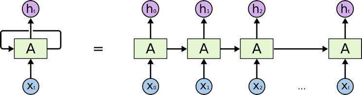
11.5. RNN
Recurrent Neural Network (RNN). A typical RNN looks like below, where X(t) is input, h(t) is output and A is the neural network which gains information from the previous step in a loop. The output of one unit goes into the next one and the information is passed.
11.5.1. Theory
from medium
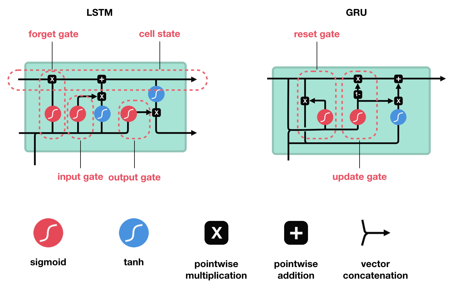
Long Short Term Memory (LSTM) is a special kind of Recurrent Neural Networks (RNN) with the capability of learning long-term dependencies. The intricacies lie within the cell, where 3 internal mechanisms called gates regulate the flow of information. This consists of 4 activation functions, 3 sigmoid and 1 tanh, instead of the typical 1 activation function. This medium from article gives a good description of it. An alternative, or simplified form of LSTM is Gated Recurrent Unit (GRU).
from medium.
11.5.2. Keras Model
LSTM requires input needs to be of shape (num_sample, time_steps, num_features) if using tensorflow backend.
This can be processed using keras’s TimeseriesGenerator.
from keras.preprocessing.sequence import TimeseriesGenerator

### UNIVARIATE ---------------------
time_steps = 6
stride = 1
num_sample = 4

X = [1,2,3,4,5,6,7,8,9,10]
y = [5,6,7,8,9,1,2,3,4,5]

data = TimeseriesGenerator(X, y,
                           length=time_steps,
                           stride=stride,
                           batch_size=num_sample)
data[0]

# (array([[1, 2, 3, 4, 5, 6],
#         [2, 3, 4, 5, 6, 7],
#         [3, 4, 5, 6, 7, 8],
#         [4, 5, 6, 7, 8, 9]]), array([2, 3, 4, 5]))
# note that y-label is the next time step away


### MULTIVARIATE ---------------------
# from pandas df
df = pd.DataFrame(np.random.randint(1, 5, (10,3)), columns=['col1','col2','label'])
X = df[['col1','col2']].values
y = df['label'].values

time_steps = 6
stride = 1
num_sample = 4

data = TimeseriesGenerator(X, y,
                           length=time_steps,
                           stride=stride,
                           batch_size=num_sample)

X = data[0][0]
y = data[0][1]
The code below uses LSTM for sentiment analysis in IMDB movie reviews.
from tensorflow.keras.preprocessing import sequence
from tensorflow.keras.models import Sequential
from tensorflow.keras.layers import Dense, Embedding
from tensorflow.keras.layers import LSTM
from tensorflow.keras.datasets import imdb

# words in sentences are encoded into integers
# response is in binary 1-0
(x_train, y_train), (x_test, y_test) = imdb.load_data(num_words=20000)

# limit the sentence to backpropagate back 80 words through time
x_train = sequence.pad_sequences(x_train, maxlen=80)
x_test = sequence.pad_sequences(x_test, maxlen=80)


# embedding layer converts input data into dense vectors of fixed size of 20k words & 128 hidden neurons, better suited for neural network
model = Sequential()
model.add(Embedding(20000, 128)) #for nlp
model.add(LSTM(128, dropout=0.2, recurrent_dropout=0.2)) #128 memory cells
model.add(Dense(1, activation='sigmoid')) #1 class classification, sigmoid for binary classification

model.compile(loss='binary_crossentropy',
            optimizer='adam',
            metrics=['accuracy'])

model.fit(x_train, y_train,
        batch_size=32,
        epochs=15,
        verbose=1,
        validation_data=(x_test, y_test))

# Train on 25000 samples, validate on 25000 samples
# Epoch 1/15
#  - 139s - loss: 0.6580 - acc: 0.5869 - val_loss: 0.5437 - val_acc: 0.7200
# Epoch 2/15
#  - 138s - loss: 0.4652 - acc: 0.7772 - val_loss: 0.4024 - val_acc: 0.8153
# Epoch 3/15
#  - 136s - loss: 0.3578 - acc: 0.8446 - val_loss: 0.4024 - val_acc: 0.8172
# Epoch 4/15
#  - 134s - loss: 0.2902 - acc: 0.8784 - val_loss: 0.3875 - val_acc: 0.8276
# Epoch 5/15
#  - 135s - loss: 0.2342 - acc: 0.9055 - val_loss: 0.4063 - val_acc: 0.8308
# Epoch 6/15
#  - 132s - loss: 0.1818 - acc: 0.9292 - val_loss: 0.4571 - val_acc: 0.8308
# Epoch 7/15
#  - 124s - loss: 0.1394 - acc: 0.9476 - val_loss: 0.5458 - val_acc: 0.8177
# Epoch 8/15
#  - 126s - loss: 0.1062 - acc: 0.9609 - val_loss: 0.5950 - val_acc: 0.8133
# Epoch 9/15
#  - 133s - loss: 0.0814 - acc: 0.9712 - val_loss: 0.6440 - val_acc: 0.8218
# Epoch 10/15
#  - 134s - loss: 0.0628 - acc: 0.9783 - val_loss: 0.6525 - val_acc: 0.8138
# Epoch 11/15
#  - 136s - loss: 0.0514 - acc: 0.9822 - val_loss: 0.7252 - val_acc: 0.8143
# Epoch 12/15
#  - 137s - loss: 0.0414 - acc: 0.9869 - val_loss: 0.7997 - val_acc: 0.8035
# Epoch 13/15
#  - 136s - loss: 0.0322 - acc: 0.9890 - val_loss: 0.8717 - val_acc: 0.8120
# Epoch 14/15
#  - 132s - loss: 0.0279 - acc: 0.9905 - val_loss: 0.9776 - val_acc: 0.8114
# Epoch 15/15
#  - 140s - loss: 0.0231 - acc: 0.9918 - val_loss: 0.9317 - val_acc: 0.8090
# Out[8]:
# <tensorflow.python.keras.callbacks.History at 0x21c29ab8630>

score, acc = model.evaluate(x_test, y_test,
                            batch_size=32,
                            verbose=1)
print('Test score:', score)
print('Test accuracy:', acc)

# Test score: 0.9316869865119457
# Test accuracy: 0.80904
This example uses a stock daily output for prediction.
from tensorflow.keras.preprocessing import sequence
from keras.preprocessing.sequence import TimeseriesGenerator
from tensorflow.keras.models import Sequential
from tensorflow.keras.layers import Dense, Embedding
from tensorflow.keras.layers import LSTM, GRU
import numpy as np
import pandas as pd
import matplotlib.pyplot as plt
import pandas_datareader.data as web
from datetime import datetime
from sklearn.preprocessing import StandardScaler
scaler = StandardScaler()
def stock(code, years_back):
end = datetime.now()
start = datetime(end.year-years_back, end.month, end.day)
code = '{}.SI'.format(code)
df = web.DataReader(code, 'yahoo', start, end)
return df
def lstm(X_train, y_train, X_test, y_test, classes, epoch, batch, verbose, dropout)
model = Sequential()
# return sequences refer to all the outputs of the memory cells, True if next layer is LSTM
model.add(LSTM(50, dropout=dropout, recurrent_dropout=0.2, return_sequences=True, input_shape=X.shape[1:]))
model.add(LSTM(50, dropout=dropout, recurrent_dropout=0.2, return_sequences=False))
model.add(Dense(1, activation='sigmoid'))
model.compile(loss='binary_crossentropy',
optimizer='adam',
metrics=['accuracy'])
model.fit(X, y,
batch_size=batch,
epochs= epoch,
verbose=verbose,
validation_data=(X_test, y_test))
return model
df = stock('S68', 10)
# train-test split-------------
df1 = df[:2400]
df2 = df[2400:]
X_train = df1[['High','Low','Open','Close','Volume']].values
y_train = df1['change'].values
X_test = df2[['High','Low','Open','Close','Volume']].values
y_test = df2['change'].values
# normalisation-------------
X_train = scaler.fit_transform(X_train)
X_test = scaler.transform(X_test)
# Conversion to keras LSTM data format-------------
time_steps = 10
sampling_rate = 1
num_sample = 1200
data = TimeseriesGenerator(X, y,
length=time_steps,
sampling_rate=sampling_rate,
batch_size=num_sample)
X_train = data[0][0]
y_train = data[0][1]
data = TimeseriesGenerator(X_test, y_test,
length=time_steps,
sampling_rate=sampling_rate,
batch_size=num_sample)
X_test = data[0][0]
y_test = data[0][1]
# model validation-------------
classes = 1
epoch = 2000
batch = 200
verbose = 0
dropout = 0.2
model = lstm(X_train, y_train, X_test, y_test, classes, epoch, batch, verbose, dropout)
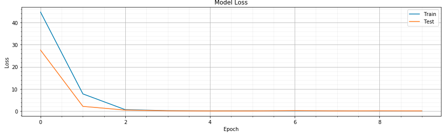
# draw loss graph
plot_validate(model, 'loss')
# draw train & test prediction
predict_train = model.predict(X_train)
predict_test = model.predict(X_test)
for real, predict in [(y_train, predict_train),(y_test, predict_test)]:
plt.figure(figsize=(15,4))
plt.plot(real)
plt.plot(predict)
plt.ylabel('Close Price');
plt.legend(['Real', 'Predict']);
Loss graph
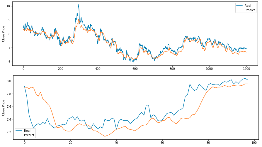
Prediction graphs
11.6. Saving the Model
From Keras documentation, it is not recommended to save the model in a pickle format. Keras allows saving in a HDF5 format. This saves the entire model architecture, weights and optimizers.
from keras.models import load_model

model.save('my_model.h5')  # creates a HDF5 file 'my_model.h5'
del model  # deletes the existing model

# returns a compiled model
# identical to the previous one
model = load_model('my_model.h5')
To save just the architecture, see https://keras.io/getting-started/faq/#how-can-i-save-a-keras-model.