14. Explainability¶

While sklearn’s supervised models are black boxes, we can derive certain plots and metrics to interprete the outcome and model better.

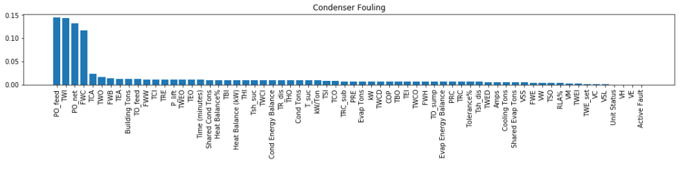
14.1. Feature Importance¶

Decision trees and other tree ensemble models, by default, allow us to obtain the importance of features. These are known as impurity-based feature importances.

While powerful, we need to understand its limitations, as described by sklearn.

they are biased towards high cardinality (numerical) features
they are computed on training set statistics and therefore do not reflect the ability of feature to be useful to make predictions that generalize to the test set (when the model has enough capacity).

import pandas as pd
from sklearn.ensemble import RandomForestClassifier

rf = RandomForestClassifier()
model = rf.fit(X_train, y_train)


import matplotlib.pyplot as plt
%config InlineBackend.figure_format = 'retina'
%matplotlib inline

def feature_impt(model, columns, figsize=(10,2)):
    '''
    desc: plot feature importance barchart for tree models
    args: model=tree model
          columns=list of column names
          figsize=chart dimensions
    returns: dataframe of feature name & their importance
    '''
    # sort feature importance in df
    f_impt= pd.DataFrame(model.feature_importances_, index=columns)
    f_impt = f_impt.sort_values(by=0,ascending=False)
    f_impt.columns = ['feature importance']

    # plot bar chart
    plt.figure(figsize=figsize)
    plt.bar(f_impt.index,f_impt['feature importance'])
    plt.xticks(rotation='vertical')
    plt.title('Feature Importance');

    return f_impt

f_impt = feature_impt(model)

14.2. Permutation Importance¶

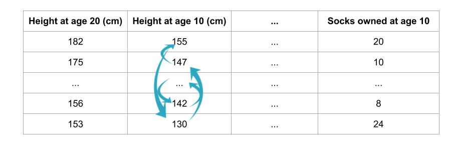
To overcome the limitations of feature importance, a variant known as permutation importance is available. It also has the benefits of being about to use for any model. This Kaggle article provides a good clear explanation

How it works is the shuffling of individual features and see how it affects model accuarcy. If a feature is important, the model accuarcy will be reduced more. If not important, the accuarcy should be affected a lot less.

From Kaggle

from sklearn.inspection import permutation_importance

result = permutation_importance(rf, X_test, y_test, n_repeats=10, random_state=42, n_jobs=2)
sorted_idx = result.importances_mean.argsort()

plt.figure(figsize=(12,10))
plt.boxplot(result.importances[sorted_idx].T,
            vert=False, labels=X.columns[sorted_idx]);

A third party also provides the same API pip install eli5.

import eli5
from eli5.sklearn import PermutationImportance

perm = PermutationImportance(my_model, random_state=1).fit(test_X, test_y)
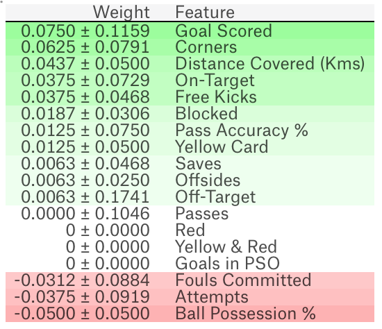
eli5.show_weights(perm, feature_names = test_X.columns.tolist())

The output is as below. +/- refers to the randomness that shuffling resulted in. The higher the weight, the more important the feature is. Negative values are possible, but actually refer to 0; though random chance caused the predictions on shuffled data to be more accurate.

From Kaggle

14.3. Partial Dependence Plots¶

While feature importance shows what variables most affect predictions, partial dependence plots show how a feature affects predictions. Using the fitted model to predict our outcome, and by repeatedly alter the value of just one variable, we can trace the predicted outcomes in a plot to show its dependence on the variable and when it plateaus.

https://www.kaggle.com/dansbecker/partial-plots

from matplotlib import pyplot as plt
from pdpbox import pdp, get_dataset, info_plots

# Create the data that we will plot
pdp_goals = pdp.pdp_isolate(model=tree_model, dataset=val_X,
                            model_features=feature_names, feature='Goal Scored')

# plot it
pdp.pdp_plot(pdp_goals, 'Goal Scored')
plt.show()

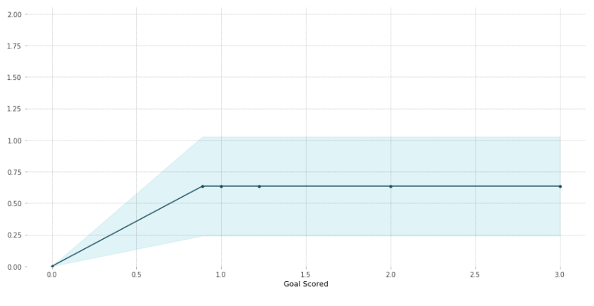
From Kaggle Learn

2D Partial Dependence Plots are also useful for interactions between features.

# just need to change pdp_isolate to pdp_interact
features_to_plot = ['Goal Scored', 'Distance Covered (Kms)']
inter1  =  pdp.pdp_interact(model=tree_model, dataset=val_X,
                            model_features=feature_names, features=features_to_plot)

pdp.pdp_interact_plot(pdp_interact_out=inter1,
                      feature_names=features_to_plot,
                      plot_type='contour')
plt.show()

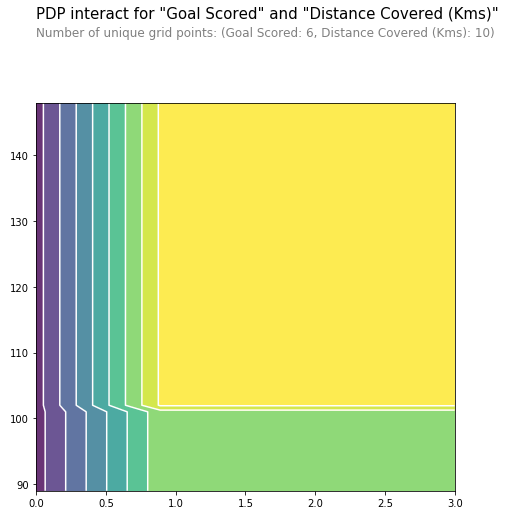
From Kaggle Learn

14.4. SHAP¶

SHapley Additive exPlanations (SHAP) break down a prediction to show the impact of each feature.

https://www.kaggle.com/dansbecker/shap-values

The explainer differs with the model type:

shap.TreeExplainer(my_model) for tree models
shap.DeepExplainer(my_model) for neural networks
shap.KernelExplainer(my_model) for all models, but slower, and gives approximate SHAP values

import shap  # package used to calculate Shap values

# Create object that can calculate shap values
explainer = shap.TreeExplainer(my_model)

# Calculate Shap values
shap_values = explainer.shap_values(data_for_prediction)

# load JS lib in notebook
shap.initjs()
shap.force_plot(explainer.expected_value[1], shap_values[1], data_for_prediction)

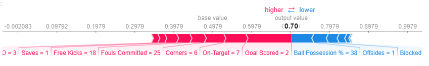
From Kaggle Learn